Around View Mapping for Advanced Driver Assistance Systems

1. Background

In autonomous driving or autonomous parking systems, surround view panorama image stitching eliminates visual blind spots around the vehicle, helping drivers intuitively assess surrounding road conditions. In this project, semantic segmentation of ground markings needs to be performed on surround view panoramic images for subsequent mapping and localization. This solution is based on four 180° fisheye cameras installed around the vehicle.

2. AVM Algorithm

2.0 Fisheye Image Correction

Based on the intrinsic calibration of fisheye cameras, fisheye camera images are corrected as shown in Figure 2.1.1.

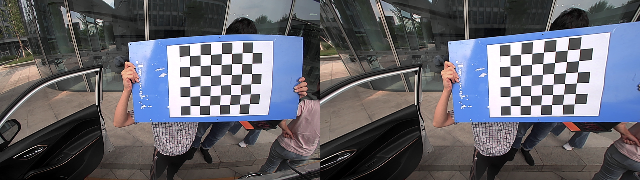
Figure 2.1.1 Fisheye Image Correction: (Left) Before correction, (Right) After correction

2.1 Top-Down Transformation

After camera-vehicle extrinsic calibration, the poses of the four surround-view cameras relative to the vehicle’s rear wheel center are obtained as \(T_{wc_1}\), \(T_{wc_2}\), \(T_{wc_3}\), and \(T_{wc_4}\). Given that the IMU is mounted at the vehicle’s rear axle center and assuming a rear axle spacing of \(d\) and axle height \(h\), the transformation from the vehicle’s left rear wheel coordinate system to the IMU coordinate system (i.e., vehicle coordinate system) is

Assuming a point \(p\) on the ground with coordinates \(p_{v}\) in the vehicle coordinate system, corresponding to homogeneous coordinates \(\tilde{p}_v\), taking the right-side camera as an example, the homogeneous coordinates of this point in the camera coordinate system can be calculated as

Using the camera intrinsic calibration matrix \(K\) and distortion model parameters \(D\) obtained through calibration, based on the fisheye camera model, \(p_{c1}\) corresponds to the fisheye image pixel coordinates \((u_{c1},v_{c1})^T\).

2.2 Surround View Image Generation

The region for generating surround view images around the vehicle is \(L\times L\). This region is rasterized into \(N\times N\) cells, where each cell corresponds to a pixel in the surround view image. Thus, the physical size of each pixel is \({L}/{N}\). Assuming the projection of the vehicle coordinate system origin’s vertical projection point on the ground corresponds to the surround view image pixel coordinates \((c_x,c_y)^T\), for any pixel point ((u,v)^T\), the corresponding 3D coordinates \(p_v\) in the vehicle coordinate system are

According to Section 2.2, the pixel coordinates \((u_{c},v_{c})^T\) corresponding to \( p_v \) on the image plane can be directly obtained. By rounding these pixel coordinates up and down, four discrete coordinate values can be obtained, denoted as \((u_{c_floor},v_{c_floor})^T\), \((u_{c_floor},v_{c_ceil})^T\), \((u_{c_ceil},v_{c_floor})^T\) and \((u_{c_ceil},v_{c_ceil})^T\). Bilinear interpolation can then be applied to obtain

Here, \(f(u_c,v_c)\) represents the image color value at pixel coordinates \((u_{c},v_{c})^T\). Thus, the color value at the coordinates \((u,v)^T\) of the surround view image is obtained, completing the generation of the surround view image.

2.3 Handling Overlapping Regions

For the 180° fisheye cameras installed around the vehicle, there are overlapping regions between each pair, as illustrated in Figure 2.3.1. Points within regions I, III, VI, and VIII may be observed by adjacent cameras simultaneously, necessitating additional fusion processing for these points.

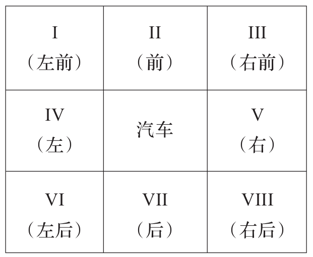
Figure 2.3.1 Vehicle Surrounding Region Division

Without loss of generality, considering region III as an example, suppose a point \((u,v)^T\) can be observed by both the right-view and front-view cameras. Its corresponding pixel coordinates on the right-view and front-view camera images are \((u_{c1},v_{c1})^T\) and \((u_{c2},v_{c2})^T\), respectively. Additionally, assume the centers of the right-view and front-view camera image planes are \((c_{x1},c_{y1})^T\) and \((c_{x2},c_{y2})^T\), respectively. Define

Based on the principle that points closer to the edges of the image exhibit more distortion, a fusion scheme for handling overlapping regions is designed as follows.

3. AVM System Implementation

3.1 AVM Algorithm Workflow

Figure 3.1.1 depicts the overall workflow of the AVM (All-round View Monitor) algorithm. It takes fisheye camera images, camera intrinsic and extrinsic parameters, and a specified AVM generation range as inputs, and outputs the AVM panoramic image. The processing includes inverse projection transformation, bilinear interpolation, and merging of overlapping regions.

graph LR
input_img(鱼眼相机图像)
input_cam(相机内外参)
output(AVM图像)
AVMcoords(AVM生成范围)
AVM2vehicle[逆向投影变换]
bilinear_interp[双线性插值]
overlap[视野重合区域融合]

AVMcoords --> AVM2vehicle 
input_cam --> AVM2vehicle 
AVM2vehicle --> bilinear_interp
input_img --> bilinear_interp
bilinear_interp --> overlap
overlap --> output

Figure 3.1.1 AVM Algorithm Workflow

The inverse projection transformation primarily maps the 3D coordinates of ground points corresponding to each pixel in the AVM panoramic image to the coordinates of the fisheye camera image plane. Discretizing the obtained pixel coordinates allows retrieval of the corresponding image color values. Subsequently, bilinear interpolation calculates the color values at the corresponding AVM image coordinates. Finally, pixels in overlapping regions between adjacent cameras are merged to produce the final AVM image result.

3.2 AVM Class Structure Design

classDiagram
	AVM <-- AVMFlow
	class AVMFlow {
	-avm_ptr_;
	-camera_info_sub_ptr;
	-image_sub_ptr;
	-avm_image_pub_ptr_;
	+ReadData();
	+HasData();
	+ValidData();
	+RunData();
	+PublishData();
	}
	class AVM {
	-trans_vehicle_wheel_;
	+Run();
	-InverseProjection();
	-BilinearInterp();
	-OverlapFusion();
	}

3.2.1 AVMFlow Class

The AVMFlow class is a data flow class adapted to the ROS interface for AVM (All-round View Monitor) stitching. It includes functionalities for reading environment camera image data and camera intrinsic/extrinsic parameter data from ROS message queues, checking the existence and validity of data, processing data, and publishing AVM stitched image data. Key methods of this class include:

bool ReadData();      // Reads data from the ROS message queue, returns true on success;
bool HasData();       // Checks if the data queue for the current time frame is non-empty, returns true if not empty;
bool ValidData();     // Checks if the latest data is valid, returns true if valid;
bool RunData();       // Executes AVM image stitching, returns true on success;
bool PublishData();   // Publishes AVM image data, returns true on success;

The main member variables of this class include:

avm_ptr_;                // Pointer to the core AVM image stitching class object;
camera_info_sub_ptr_;    // Pointer for receiving camera intrinsic/extrinsic parameter data;
image_sub_ptr_;          // Pointer for receiving environment camera image data;
avm_image_pub_ptr_;      // Pointer for publishing AVM image data;

3.2.2 AVM Class

The AVM class is the core processing class for AVM image stitching. It includes functionalities for inverse projection of observed ground ranges into AVM panoramic images, bilinear interpolation of AVM image color values, and fusion processing of overlapping regions between adjacent cameras. Key methods of this class include:

bool Run();                // Core function external interface;
bool InverseProjection();  // Functionality for inverse projection;
bool BilinearInterp();     // Bilinear interpolation function;
bool OverlapFusion();      // Overlap region fusion function;

The main member variables of this class include:

trans_vehicle_wheel_;   // Transformation from the calibration cross coordinate system to the vehicle coordinate system;

4. Adaptive IPM Algorithm

4.1 Algorithm Principles

When generating AVM images using calibrated camera-to-vehicle extrinsics, it is necessary to ensure that the vehicle coordinate system’s OXY plane remains parallel to the ground. However, during vehicle acceleration, deceleration, and when passing over speed bumps, it is challenging to maintain this parallelism. Therefore, the adaptive IPM algorithm compensates for the vehicle’s attitude using the pitch angle \(\theta\) and roll angle \(\varphi\) provided by the integrated navigation system.

In the adaptive IPM algorithm, assuming the integrated navigation system provides the vehicle’s pitch angle \(\theta\) and roll angle \(\varphi\), the required compensatory rotational transformation in the vehicle coordinate system is determined based on the vehicle’s coordinate system settings.

After compensation, the transformation from the vehicle coordinate system to the vehicle rear wheel (calibration cloth) coordinate system is

4.2 Debugging Records

When traversing between different areas of the parking lot, noticeable compensation effects are observed due to significant slopes, as shown in Figure 4.2.1.

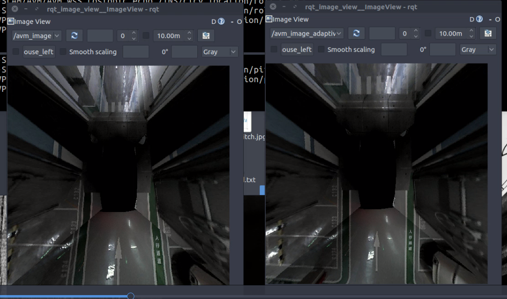
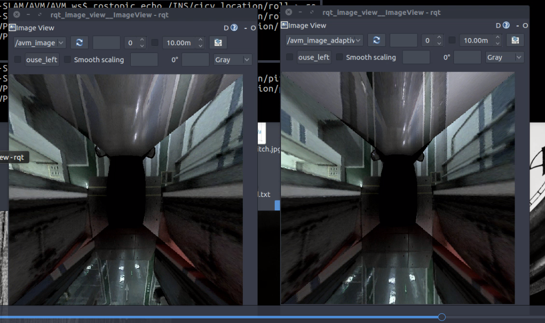
Figure 4.2.1: Adaptive IPM algorithm compensation effect in an underground parking lot: (Left) Before compensation, (Right) After compensation.

When the vehicle passes over speed bumps, it is difficult to visually assess the compensation effect. The pitch angle variation curve is shown in Figure 4.2.2, where the three larger peaks correspond to the process of entering and exiting slopes in the parking lot, and the four pulses in the middle correspond to the connection between parking lot areas. There is no specific waveform clearly corresponding to speed bumps.

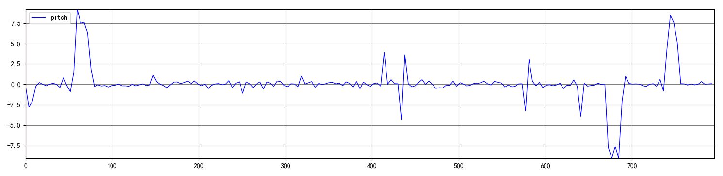
Figure 4.2.2: Pitch angle variation curve in an underground parking lot.

The curve of pitch angle and its corresponding observation variance is shown in Figure 4.2.3. Except for the specific waveforms mentioned earlier, the fluctuations in other parts of the curve are mostly within the variance range. In other words, they are likely caused by noise, indicating that using them for vehicle attitude compensation may not be meaningful.

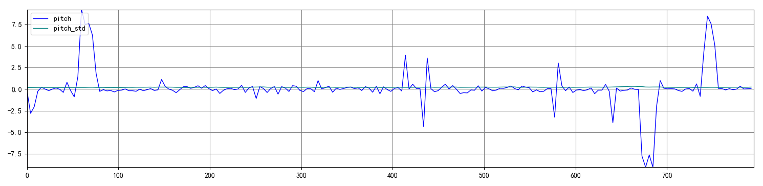
Figure 4.2.3: Pitch angle and its variance variation curve in an underground parking lot.

In summary, the attitude estimation results provided by the integrated navigation system can only be used to compensate for significant tilt changes in the vehicle’s attitude. They are not sufficiently accurate for compensating for normal road vibrations, passing over speed bumps, or changes in vehicle acceleration and deceleration.

5.Results

5.1 Scenario One: Underground Parking Lot

5.2 Scenario Two: Open Roadways

6.Related Links

code:

• avm