Magnetic Interference Compensation Based on Ellipsoid Fitting
Date:
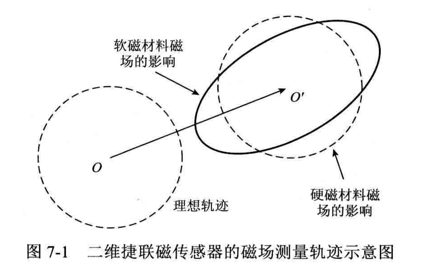
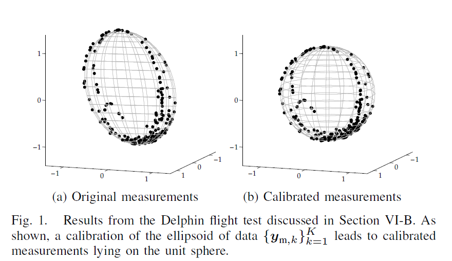
Under the condition of no errors and interference, when the carrier rotates in a uniform magnetic field, the magnitude of the measured magnetic field vector is not affected by the attitude, and its trajectory falls on a spherical surface in three-dimensional space. When errors and interference are present, theoretically, the trajectory of the measured magnetic field vector forms an ellipsoidal surface.
Magnetometer measurement model
The measurement model of the magnetometer-inertial navigation system is
\[\boldsymbol{y}_{k}^m=C_{sc}C_{no} (C_{si}\boldsymbol{m}_k^m+\boldsymbol{o}_{hi}) +\boldsymbol{o}_{zb}+\boldsymbol{e}_{k}^m\]where
\(\boldsymbol{y}_{k}^m\) is the magnetic field measurement data;
\(\boldsymbol{m}_k^m\) is the geomagnetic vector represented in the magnetometer frame;
\(C_{sc}\) is the magnetometer triaxial sensitivity matrix;
\(C_{no}\) is the magnetometer triaxial non-orthogonal matrix;
\(\boldsymbol{o}_{zb}\) is the magnetometer triaxial zero bias;
\(\boldsymbol{e}_{k}^m\) is the measurement noise of the magnetometer;
\(C_{si}\) is the induced magnetic field matrix in the carrier interference field (soft-iron effect);
\(\boldsymbol{o}_{hi}\) is the fixed magnetic field vector in the carrier interference field (hard-iron effects).
After further organization, the final measurement model is obtained as follows.
\[\boldsymbol{y}_{k}^m=D\boldsymbol{m}_k^m+\boldsymbol{o}+\boldsymbol{e}_{k}^m\]where
\[D=C_{sc}C_{no}C_{si}\] \[\boldsymbol{o}=C_{sc}C_{no}\boldsymbol{o}_{hi}+\boldsymbol{o}_{zb}\]The above model is relatively common in current research. Some assumptions for the model to hold include:
The interference magnetic field must come from equipment or carrier platforms rigidly attached to the sensor.
During calibration data collection, the external magnetic field (geomagnetic field) is uniform and constant.
In this study, both assumptions can be considered as satisfied.
Quadrics
Quadratic surfaces include different shapes such as spheres, ellipsoids, and paraboloids. The general form of the quadratic surface equation can be expressed as
\[S: ax^2+by^2+cz^2+2fyz+2gxz+2hxy+2px+2qy+2rz+d=0.\]The matrix form of the above equation is represented by
\[S: \boldsymbol{x}^T\boldsymbol{M}\boldsymbol{x}+ 2\boldsymbol{n}^T\boldsymbol{x}+d=0\]where
\[\boldsymbol{x}= \begin{bmatrix} x\\ y\\ z \end{bmatrix}\] \[\boldsymbol{M}= \begin{bmatrix} a & h & g \\ h & b & f \\ g & f & c \\ \end{bmatrix}\] \[\boldsymbol{n}= \begin{bmatrix} p\\ q\\ r \end{bmatrix}\]Ellipsoid fit
First, let \(\mathcal{F}\) represent the uniform geomagnetic field strength in the area where the carrier is located, that is,
\[\|{m}^n\|_2=\mathcal{F}\]Then the following equation holds.
\[\|{m}^n\|_2^2-\mathcal{F}^2=\|R_k^{nm}{m}_k^m\|_2^2-\mathcal{F}^2=\|{m}_k^m\|_2^2-\mathcal{F}^2=0\]Expanding this, we obtain the ellipsoid constraint equation as follows.
\[\begin{aligned} 0&=\|D^{-1}({y}_{k}^m-{o}-{e}_{k}^m)\|_2^2-\mathcal{F}^2 \\ &\approx{y_{k}^m}^TA{y}_{k}^m+2{b}^T{y}_{k}^m+c \end{aligned}\]where
\[A=D^{-T}D^{-1} \tag{1}\] \[{b}^T=-{o}^TD^{-T}D^{-1} \tag{2}\] \[c={o}^TD^{-T}D^{-1}{o}-\mathcal{F}^2 \tag{3}\]Ellipsoid fitting can refer to the method proposed in reference 1 and its corresponding MATLAB implementation 2. Using the ellipsoid fitting method, estimates \(\hat{A}_s,\hat{b}_s,\hat{c}_s\) of the ellipsoid coefficients can be obtained.
From the ellipsoid equation, it can be observed that for any \(\alpha\in\mathbb{R}\),\(\alpha\hat{A}_s,\alpha\hat{b}_s,\alpha\hat{c}_s\) also satisfy the ellipsoid equation.
\[\begin{aligned} \mathcal{F}^2&={o}^TD^{-T}D^{-1}{o}-c \\ &=b^TA^{-1}b-c \\ &=\alpha(\hat{b}_s^T\hat{A}_s^{-1}\hat{b}_s-\hat{c}_s) \end{aligned}\]According to the constraint provided by equation (3), the value of the variable \(\alpha\) can be determined.
\[\alpha=(\hat{b}_s^T\hat{A}_s^{-1}\hat{b}_s-\hat{c}_s)^{-1}\mathcal{F}^2\]Next, based on equations (1)-(3), the estimated model parameters \(\hat{D},\hat{o}\) are solved.
\[\hat{D}^{-T}\hat{D}^{-1}=\alpha\hat{A}_s \tag{4}\] \[\hat{o}=-\hat{A}_s^{-1}\hat{b}_s\]According to equation (4), it can be seen that \(\hat{D}\) does not have a unique solution because for any matrix \(V\) satisfying \(V^TV=I_3\), \(\hat{D}V\) can satisfy equation (4).
By performing an eigenvalue decomposition on the right-hand side of equation (4), we can obtain a particular solution denoted as \(\tilde{D}\).
\[\begin{aligned} (\tilde{D}^{-1})^T(\tilde{D}^{-1}) &=\alpha U\Lambda U^T =\alpha U\Lambda^{1/2}\Lambda^{1/2} U^T \\ &=\alpha (\Lambda^{1/2} U^T)^T(\Lambda^{1/2} U^T) \end{aligned}\] \[\tilde{D}^{-1}=\sqrt{\alpha}\Lambda^{1/2} U^T\]Therefore, the relationship between \(\tilde{D}\) and the final solution \(\hat{D}\) is
\[\hat{D}=\tilde{D}V\]The unknown orthogonal matrix \(V\) here represents the alignment relationship between the magnetometer and the inertial navigation system, and cannot be determined solely through magnetic measurement data 3.
Alignment with Inertial Sensor
The geomagnetic vector \(\boldsymbol{m}_k^m\) represented in the magnetometer frame relates to the geomagnetic vector in the navigation frame as
\[\boldsymbol{m}_k^m=R_k^{mn}\boldsymbol{m}^n=R^{mb}R_k^{bn}\boldsymbol{m}^n \tag{5}\]Where:
- \(R^{mb}\) represents the attitude transformation from the body frame to the magnetometer frame,
- \(R_k^{bn}\) represents the attitude of the body frame in the navigation frame at time \(k\).
From equation (5), it can be seen that when the carrier moves in a uniform geomagnetic field for calibration, the variation in the measured magnetic field vector depends solely on the changes in the carrier’s attitude 4.
Substituting the solved results of the previous section’s model parameters and equation (5) into the measurement model, we obtain
\[\begin{aligned} \boldsymbol{y}_{k}^m&=\hat{D}\boldsymbol{m}_k^m+\hat{o} \\ &=\tilde{D}VR^{mb}R_k^{bn}\boldsymbol{m}^n+\hat{o} \end{aligned}\]let
\[R=VR^{mb}\]then
\[\boldsymbol{y}_{k}^m=\tilde{D}RR_k^{bn}\boldsymbol{m}^n+\hat{o} \tag{6}\]For the next time step \(k+1\), the observed data are given by
\[\boldsymbol{y}_{k+1}^m=\tilde{D}RR_{k+1}^{bn}\boldsymbol{m}^n+\hat{o} \tag{7}\]Combining equations (6) and (7), we obtain
\[\boldsymbol{y}_{k+1}^m=\tilde{D}RR_{k+1}^{bn} R_k^{nb}R^T\tilde{D}^{-1}(\boldsymbol{y}_{k}^m-\hat{o}) +\hat{o}\]let
\[R^{b_{k+1}}_{b_k}=R_{k+1}^{bn}R_k^{nb}\]then we have
\[\boldsymbol{y}_{k+1}^m=\tilde{D}R R^{b_{k+1}}_{b_k} R^T\tilde{D}^{-1}(\boldsymbol{y}_{k}^m-\hat{o}) +\hat{o} \tag{8}\]Equation (8) provides the relationship between the attitude increment \(R^{b_{k+1}}_{b_k}\) provided by the inertial navigation system between two time steps, and the correlation between the observations of the triaxial vector magnetometer.
Initial Value Estimation
If there is no suitable initial value, a nonlinear optimization problem may fail to converge to a global optimal solution. Therefore, an initial value is estimated for the alignment problem stated above. Eqn.(6) can be rewritten as
\[\tilde{D}^{-1}(\boldsymbol{y}_{k}^m-\hat{o})=RR_k^{bn}\boldsymbol{m}^n\]Let
\[\begin{aligned} & p_k'\triangleq\tilde{D}^{-1}(\boldsymbol{y}_{k}^m-\hat{o}) \\ & p_k\triangleq R_k^{bn}\boldsymbol{m}^n \end{aligned}\]Then, a minimization problem is constructed as
\[\min_{R}\sum_k\|p_k'-Rp_k\|^2 \tag{9}\]Compute the mean values of \(p_k’\) and \(p_k\), respectively, and define
\[\begin{aligned} & q_k'\triangleq p_k'-{\rm mean}(p_k') \\ & q_k\triangleq p_k-{\rm mean}(p_k) \end{aligned}\]The minimization problem (9) is reconstructed as
\[\min_{R}\sum_k\|q_k'-Rq_k\|^2 \tag{9}\]Define matrix \(H\)5 as
\[H\triangleq\sum_k q_k'q_k^T\]Compute the singular value decomposition (SVD) of the matrix \(H\) as
\[H=U\Lambda V^T\]Then, the orthogonal matrix \(\hat{R}\) that minimized (9) can be calculated by 5
\[\hat{R}=VU^T\]Magnetometer outside Cabin
The measurements of the magnetometer outside the cabin are denoted by the superscript \(m’\).
\[\begin{aligned} \boldsymbol{y}_{k}^m&=\hat{D}\boldsymbol{m}_k^m+\hat{o} \\ &=\tilde{D}VR^{mm'}\boldsymbol{m}^{m'}_k+\hat{o} \end{aligned}\]let
\[R=VR^{mm'}\]then
\[\boldsymbol{y}_{k}^m=\tilde{D}R\boldsymbol{m}^{m'}_k+\hat{o} \tag{10}\]Rewriting Eqn.(10) yields
\[\tilde{D}^{-1}(\boldsymbol{y}_{k}^m-\hat{o})=R\boldsymbol{m}^{m'}_k\]Let
\[\begin{aligned} & p_k'\triangleq\tilde{D}^{-1}(\boldsymbol{y}_{k}^m-\hat{o}) \\ & p_k\triangleq \boldsymbol{m}^{m'}_k \end{aligned}\]Then, the initial value estimation method mentioned above can be applied here. Given an initial value, the ceres optimization problem can be constructed to solve Eqn.(10).
Experiments
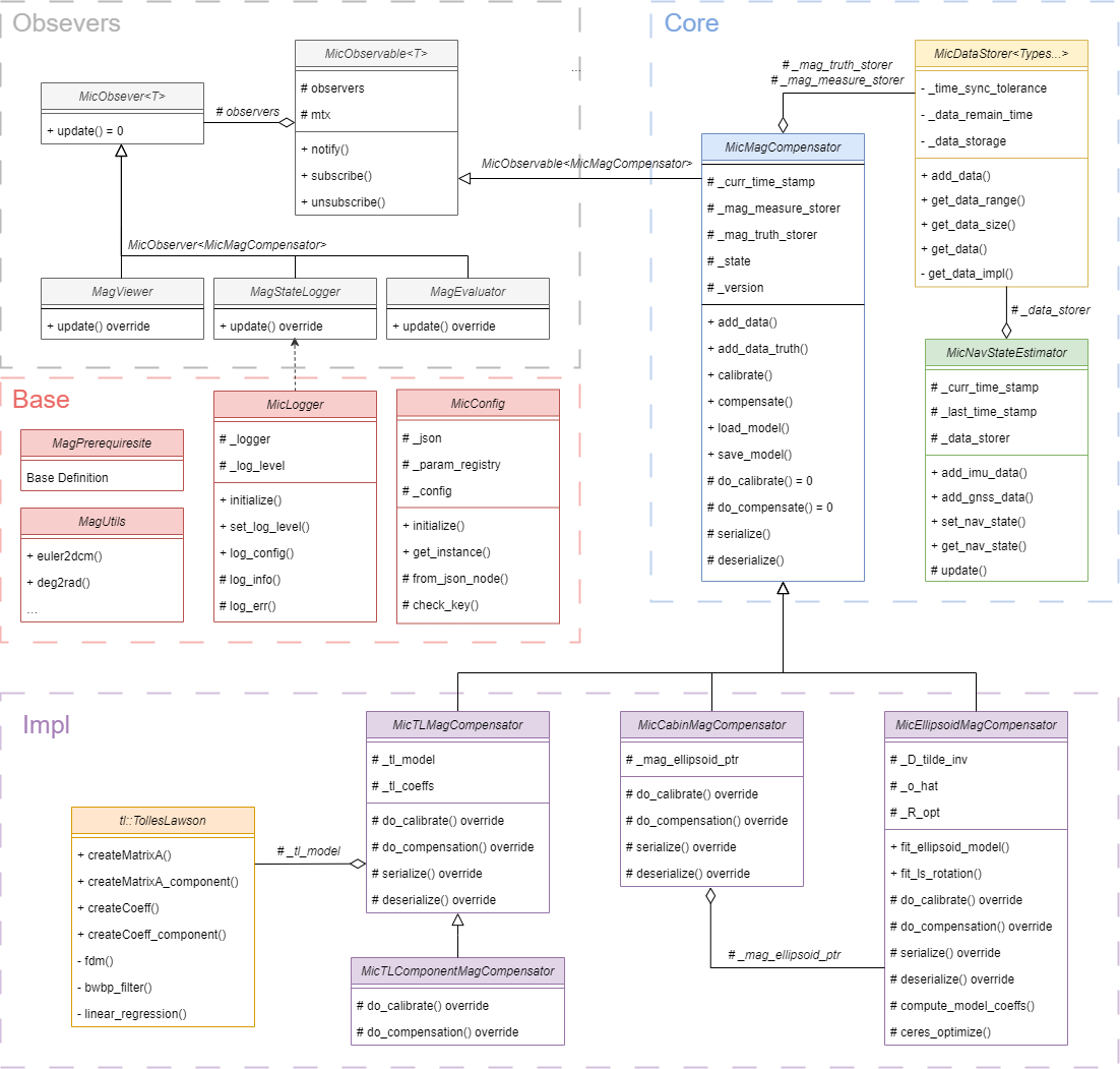
Framework
Flight 1002
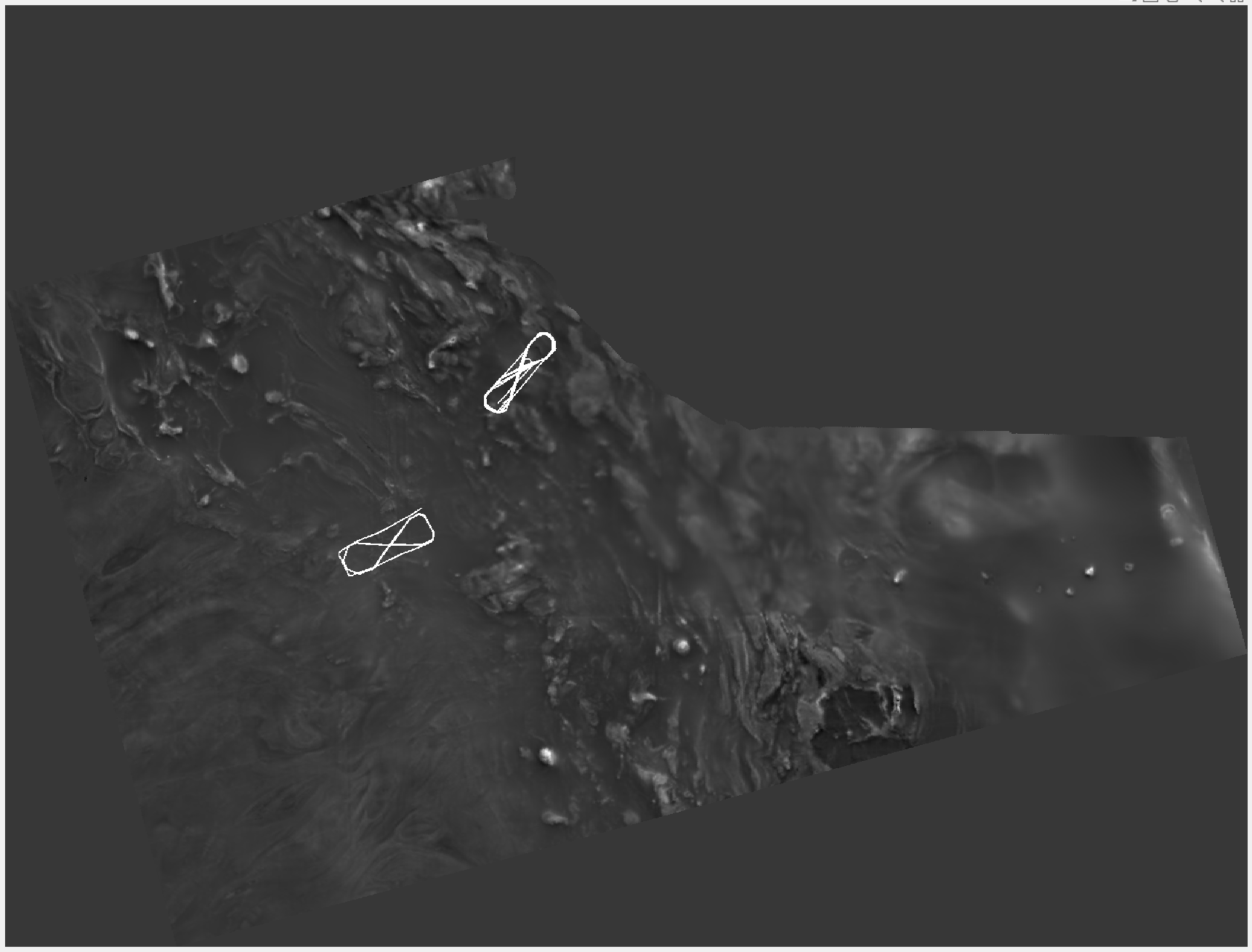
The relevant information regarding this flight route can be found in Flt1002_readme.txt. For the experiment, select data collected from calibration flight paths 1002.02 and 1002.20. Plot these two calibration flight paths in the anomaly map as shown below.
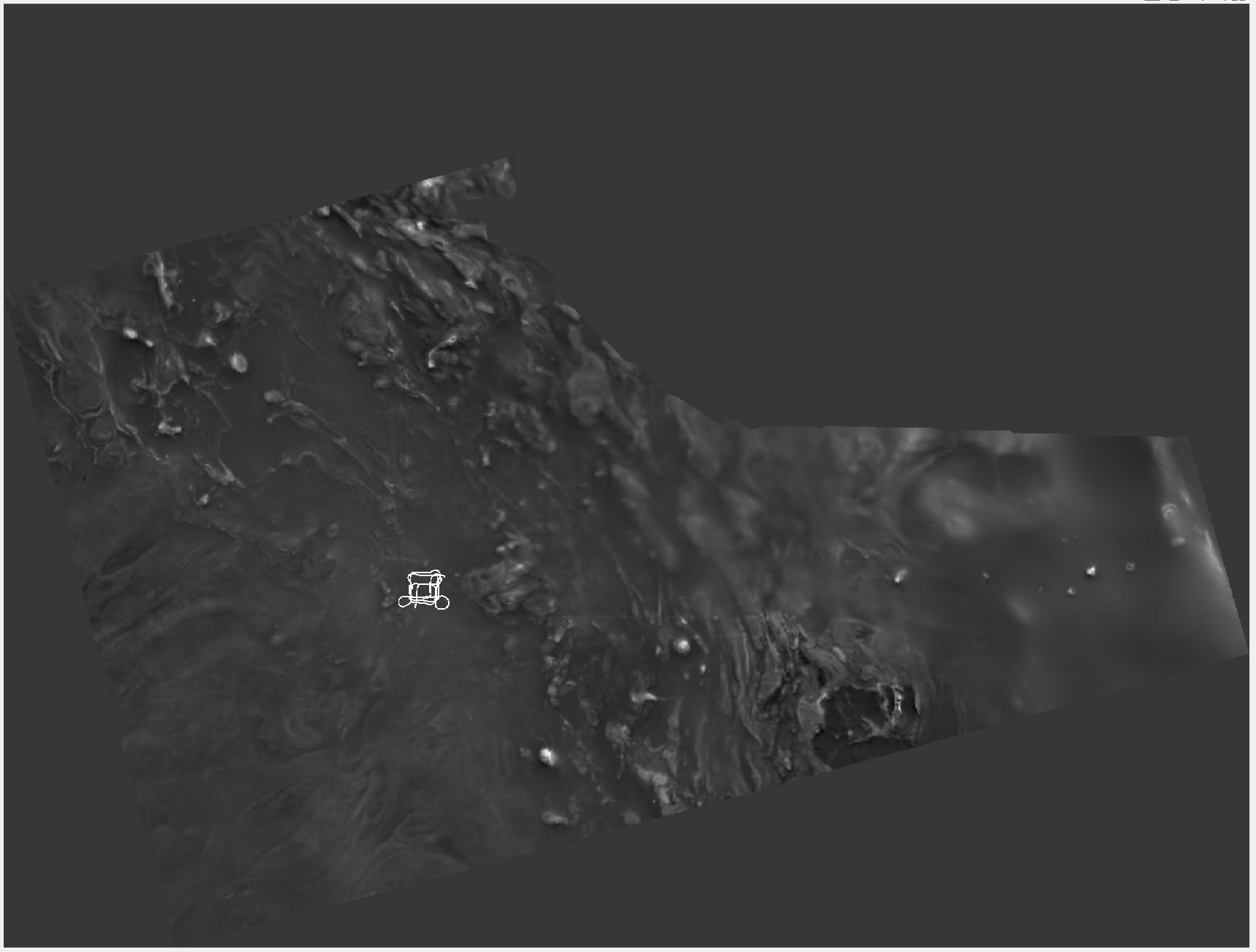
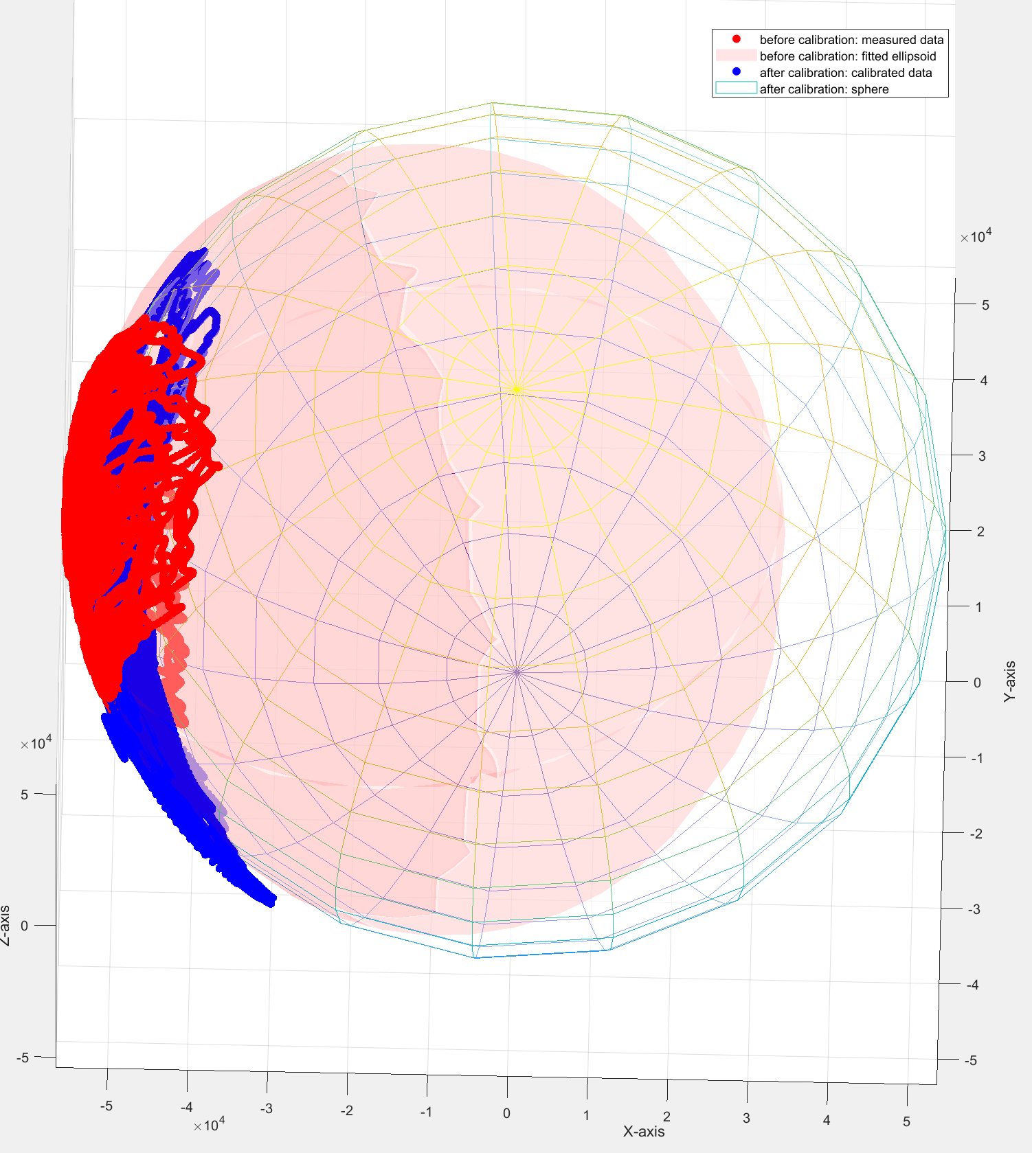
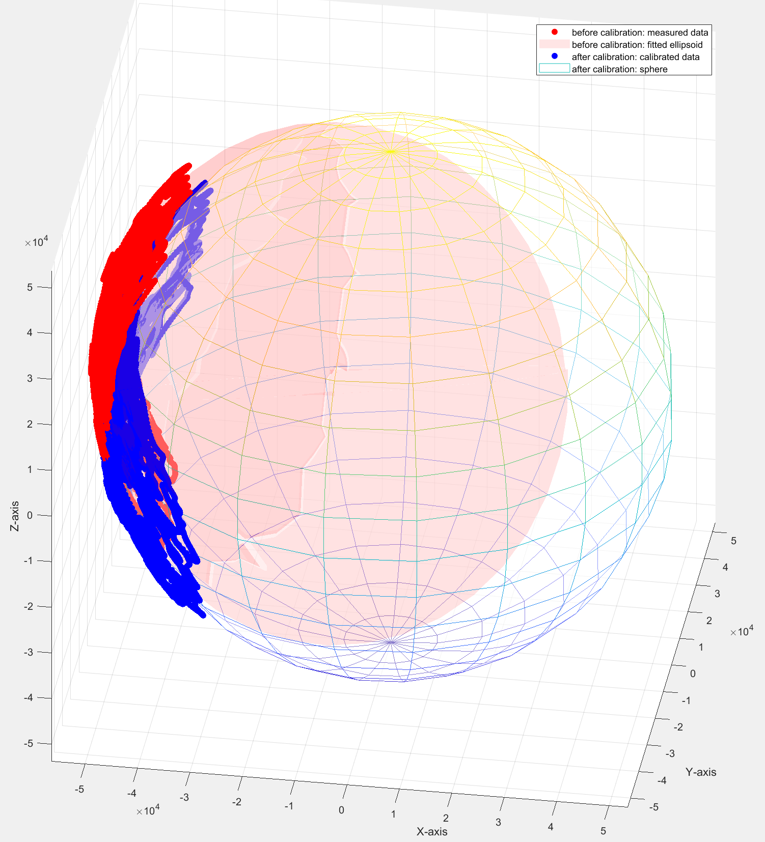
The calibration results can be seen from the figure below.
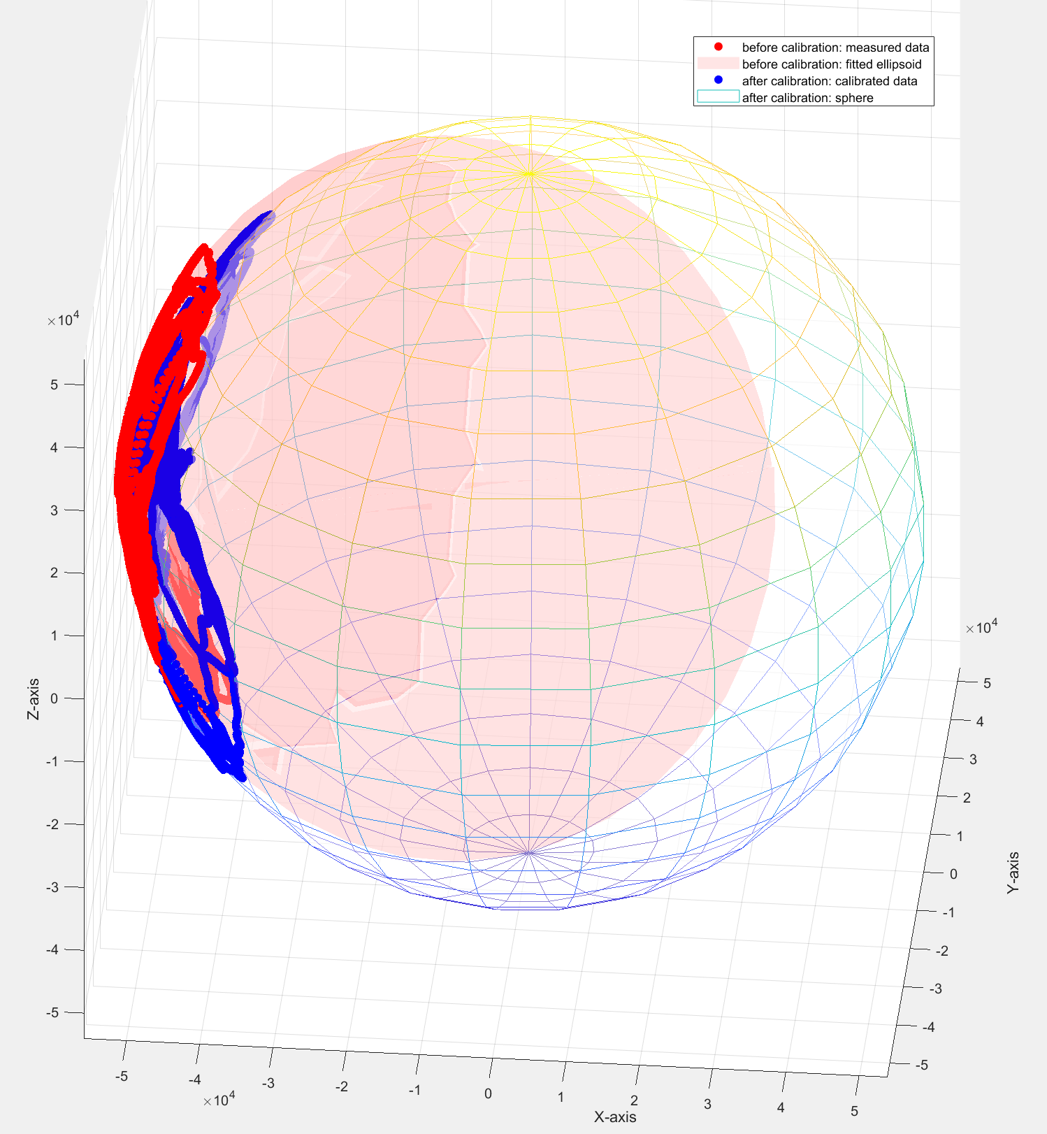
The RMSE errors before and after correction are shown in the following table.
| Before Correction | After Correction | |
|---|---|---|
| RMSE | 1665.04 nT | 82.57 nT |
Flight 1003
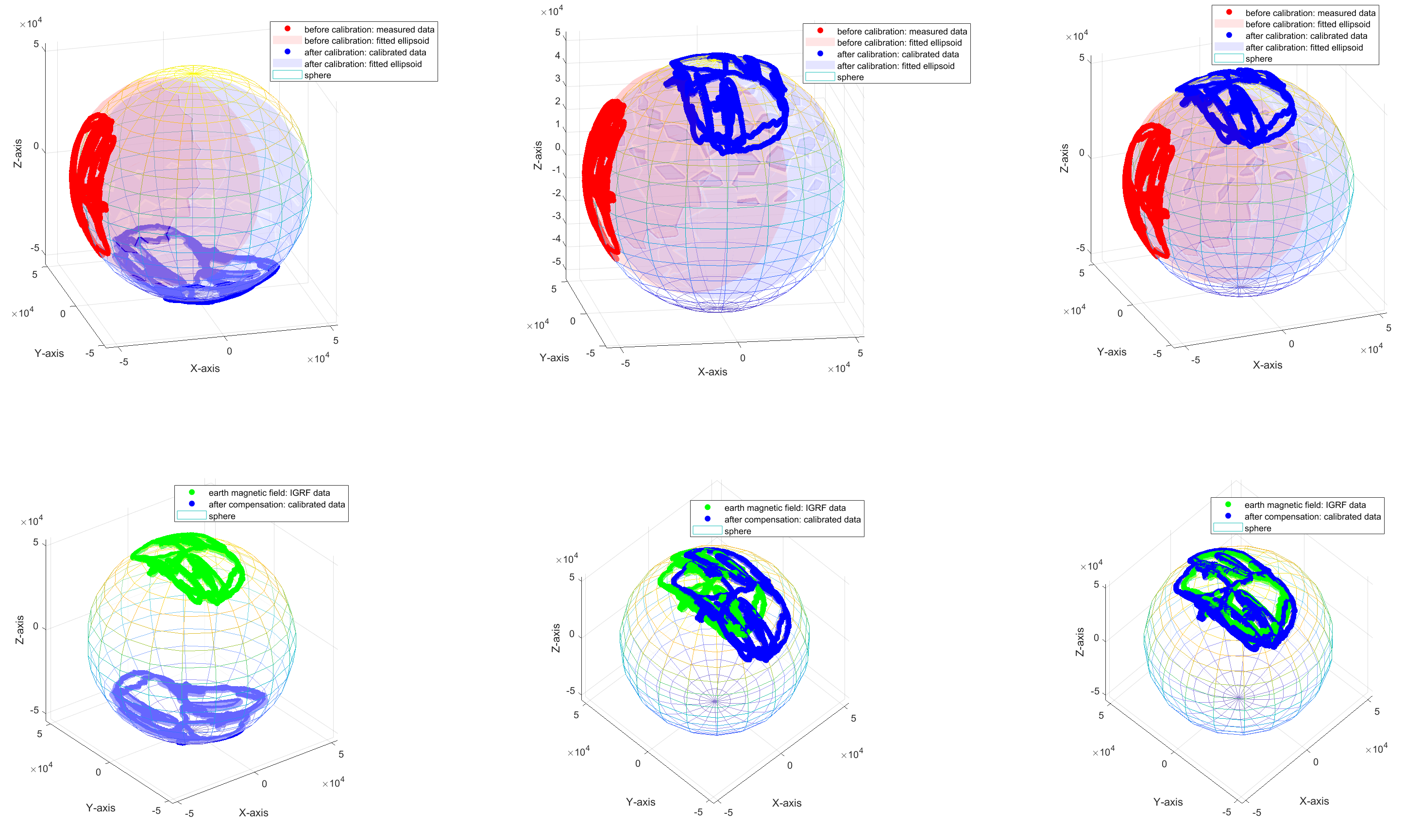
The model parameters calculated using the calibration flight data from Flight 1002 are applied to correct Flight 1003. The results are verified using data from flights 1003.02, 1003.04, and 1003.08. Plot these three calibration flight paths in the anomaly map as shown in the following figure.
The calibration results can be seen from the figure below.
| Before Correction | After Correction | |
|---|---|---|
| RMSE | 2316.71 nT | 688.72 nT |
Experiments for Alignment with INS
1002.02
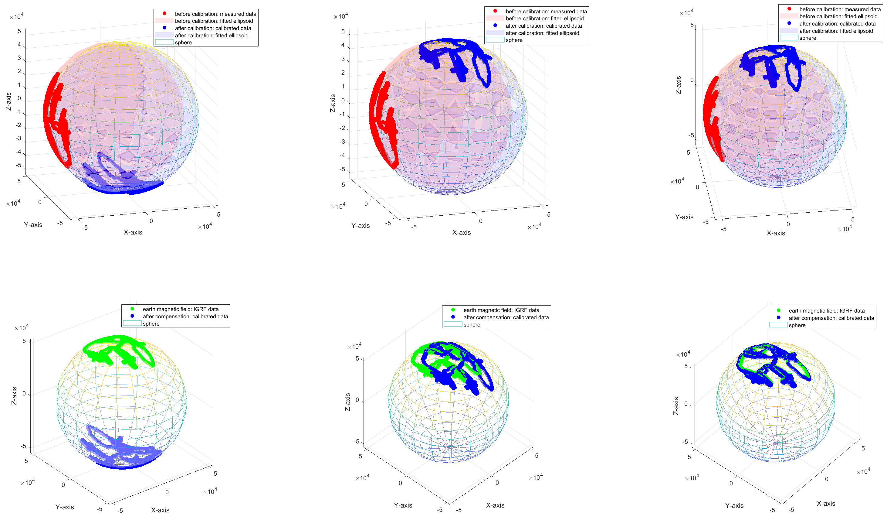
1002.20
Statement
This work has been submitted to the IEEE for possible publication. Copyright may be transferred without notice, after which this version may no longer be accessible.
© 20xx IEEE. Personal use of this material is permitted. Permission from IEEE must be obtained for all other uses, including reprinting/republishing this material for advertising or promotional purposes, collecting new collected works for resale or redistribution to servers or lists, or reuse of any copyrighted component of this work in other works.
Related Links
code: