3D NDT
Published:
reading notes.
3D NDT (PhD thesis of M. Magnusson)
This quotations in this section is mainly from the Doctoral thesis “The three-dimensional normal-distributions transform: an efficient representation for registration, surface analysis, and loop detection” of Dr. Martin Magnusson
The normal-distributions transform can be described as a method for compactly representing a surface. It was first proposed by Biber and Straßer in 2003 [7] as a method for 2D scan registration. Biber and Straßer later elaborated on the method in a joint paper with Sven Fleck [8], also in the context of scan registration and mapping.
[7] Peter Biber and Wolfgang Straßer. The normal distributions transform: A new approach to laser scan matching. In Proceedings of the IEEE International Conference on Intelligent Robots and Systems (IROS), pages 2743–2748, Las Vegas, USA, October 2003.
[8] Peter Biber, Sven Fleck, and Wolfgang Straßer. A probabilistic framework for robust and accurate matching of point clouds. In 26th Pattern Recognition Symposium (DAGM 04), 2004.
Assuming that the locations of the reference scan surface points were generated by a D-dimensional normal random process, the likelihood of having measured \(\vec{x}\) is
\[p(\vec{x})= \frac{1}{(2\pi)^{D/2}\sqrt{|\Sigma|}} \exp \left( -\frac{(\vec{x}-\vec{\mu})^T\Sigma^{-1}(\vec{x}-\vec{\mu})}{2} \right)\]When using NDT for scan registration, the goal is to find the pose of the current scan that maximises the likelihood that the points of the current scan lie on the reference scan surface.
\[\Psi=\prod^{n}_{k=1}p(T(\vec{p},\vec{x}_k))\]Assume that there is a spatial transformation function \(T(\vec{p},\vec{x})\) that moves a point \(\vec{x}\) in space by the pose \(\vec{p}\). Given some PDF \(p(\vec{x})\) for scan points, the best pose should be the one that maximises the likelihood function
\[-\log\Psi=-\sum^{n}_{k=1}\log p(T(\vec{p},\vec{x}_k))\]or, equivalently, minimises the negative log-likelihood of \(\Psi\):
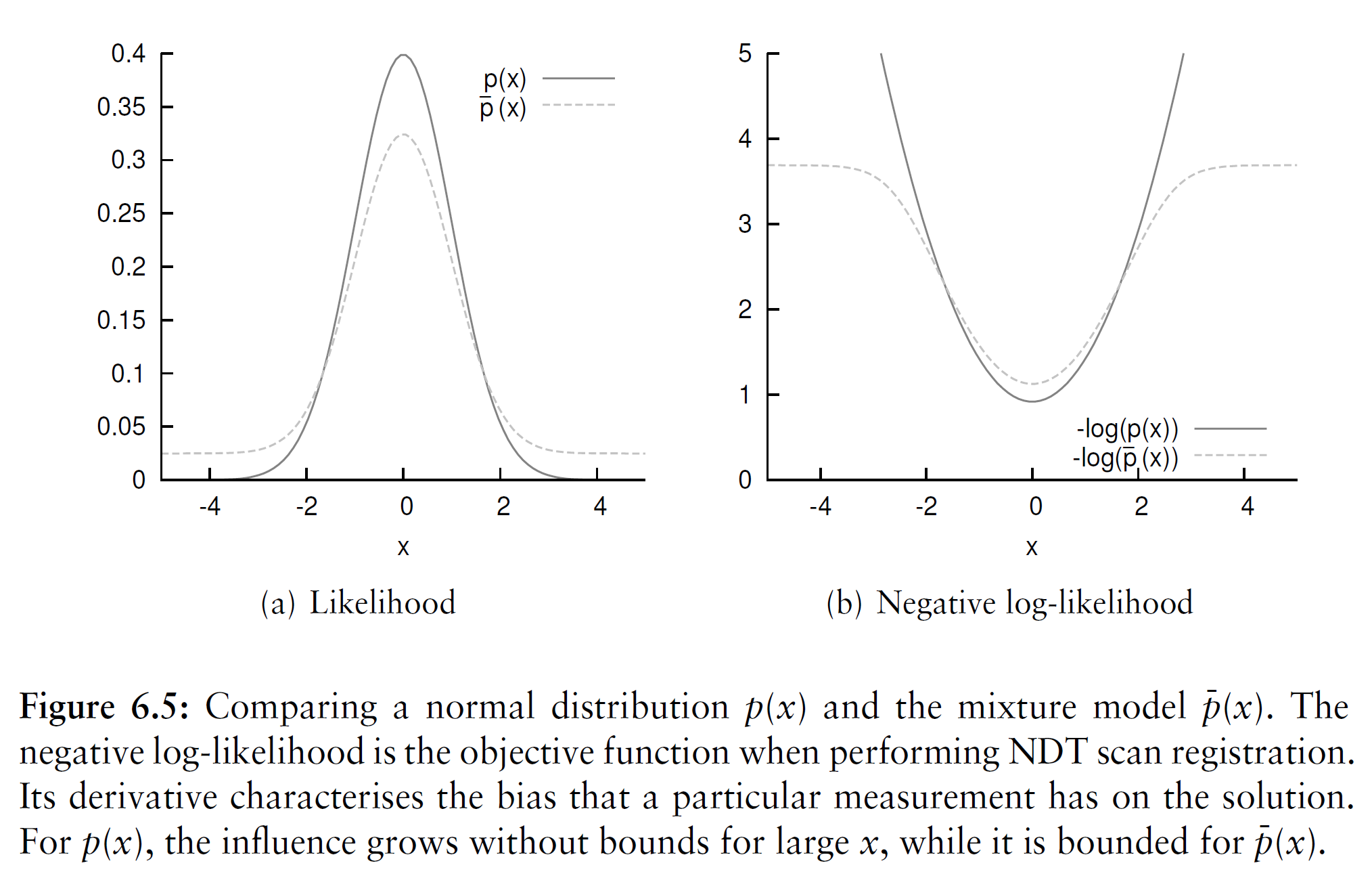
\[\bar{p}(\vec{x})= c_1 \exp \left( -\frac{(\vec{x}-\vec{\mu})^T\Sigma^{-1}(\vec{x}-\vec{\mu})}{2} \right) +c_2p_0\]The PDF is not necessarily restricted to be a normal distribution. Any PDF that locally captures the structure of the surface points and is robust to outliers is suitable. The negative log-likelihood of a normal distribution grows without bound for points far from the mean. Consequently, outliers in the scan data may have a large influence on the result. In this work (as in the paper by Biber, Fleck, and Straßer [8]) a mixture of a normal distribution and a uniform distribution is used:
where \(p_0\) is the expected ratio of outliers. Using this function, the influence of outliers is bounded. This is illustrated in Figure 6.5. The constants \(c_1\) and \(c_2\) can be determined by requiring that the probability mass of \(\bar{p}(\vec{x})\) equals one within the space spanned by a cell.

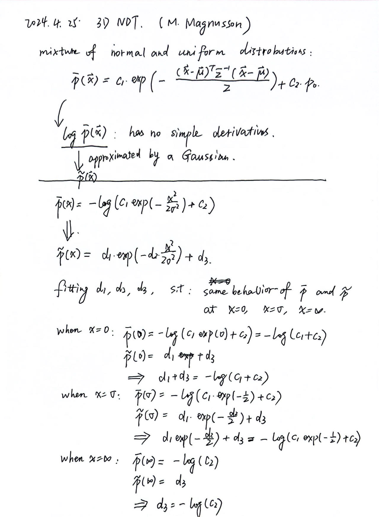
\[\bar{p}(x)= -\log \left( c_1 \exp \left( -\frac{x^2}{2\sigma^2} \right) +c_2 \right)\]The summands of the log-likelihood energy function to be optimised consist of terms that have the form \(−\log(c_1\exp(\cdot)+c_2)\). These have no simple first- and second-order derivatives. However, Figure 6.5(b) suggests that the log-likelihood function can, in turn, be approximated by a Gaussian. A function on the form
\[\tilde{p}(x)= d_1 \exp \left( -\frac{d_2x^2}{2\sigma^2} \right) +d_3\]may be approximated by a Gaussian
\[\begin{aligned} & d_3=-\log(c_2) \\ & d_1=-\log(c_1+c_2)-d_3 \\ & d_2=-2\log \frac{-\log(c_1\exp(-1/2)+c_2)-d_3}{d_1} \end{aligned}\]fitting the parameters \(d_i\) by requiring that \(\tilde{p}(x)\) should behave like \(\bar{p}(x)\) for \(x = 0\), \(x = σ\), and \(x = ∞\).

\[\tilde p(\vec{x}_k)= -d_1 \exp \left( -\frac{d_2}{2}(\vec{x}_k-\vec{\mu}_k)^T\Sigma_k^{-1}(\vec{x}_k-\vec{\mu}_k) \right)\]Using such a Gaussian approximation, the influence of one point from the current scan on the NDT score function is
This NDT score function has simpler derivatives than the logarithm of mixed distribution but still exhibits the same general properties when used in optimisation. Note that the \\(d_3\\) term has been omitted. It is not required when using NDT for scan registration, since it only adds a constant offset to the score function, and does not change its shape or the parameters for which it is optimised.
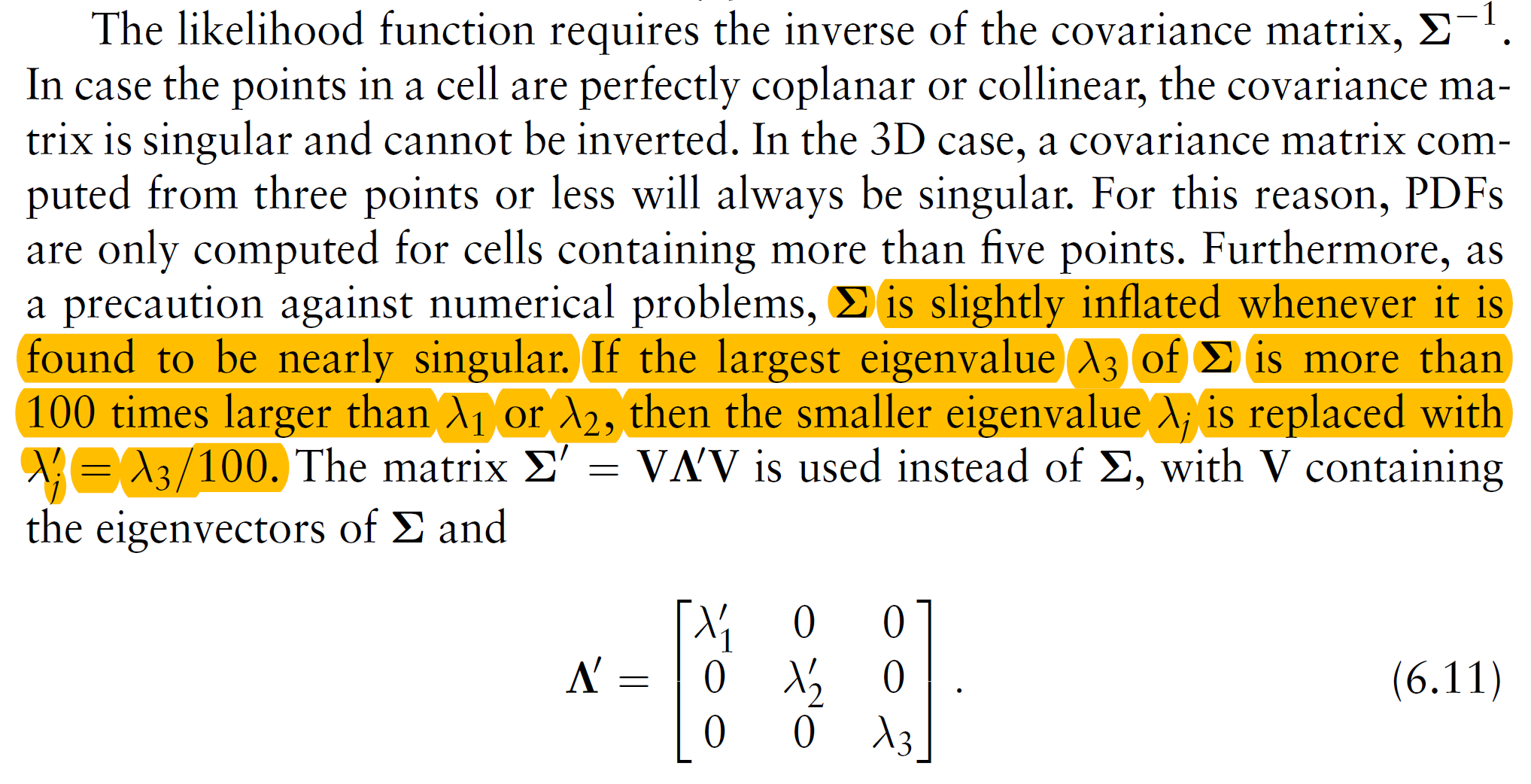
some manipulations about the covariance (does the inflation possibly affect the calculation of degeneration):

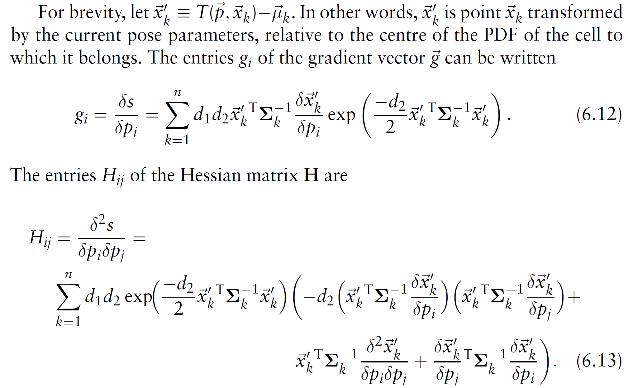
An overall formulation of the gradient vector and Hessian matrix:
