Semantic GICP-based Point Cloud Registration
Date:
GICP Point Cloud Registration
GICP
Similar to traditional ICP, Euclidean distance is used in the nearest point search, facilitating acceleration of the search process using kd-tree. Suppose two ordered sets of points denoted by
\[A=\{a_i\}_{i=1,\dots,N}\] \[B=\{b_i\}_{i=1,\dots,N}\]where \(a_i\) and \(b_i\) represent a pair of associated points.
Assume these two sets of points are sampled from Gaussian probability distributions, i.e., \(a_i \sim \mathcal{N}(\hat{a}_i, C^A_i)\) and \(b_i \sim \mathcal{N}(\hat{b}_i, C^B_i)\). For the correct sensor pose transformation \(T^*\), there exists
\[\hat{b}_i=T^*\hat{a}_i\]For an unoptimized pose transformation \(T\), define the residual \(d_i(T) = b_i - T a_i\). Since \(a_i\) and \(b_i\) are sampled from mutually independent Gaussian distributions, it follows that
\[\begin{aligned} d_i(T^*)&\sim\mathcal{N} \left(\hat{b}_i-T^*\hat{a}_i,C_i^B+T^*C_i^AT^{*T}\right)\\ &=\mathcal{N} \left(0,C_i^B+T^*C_i^AT^{*T}\right) \end{aligned}\]Then, MLE are used to solve \(T\).
\[\begin{aligned} T=&\arg\max_T\prod_ip(d_i(T)) =\arg\max_T\sum_i\log(p(d_i(T)))\\ &\arg\min_T \sum_i d_i(T)^T (C_i^B+TC_i^BT^T)^{-1} d_i(T)\\ \end{aligned}\]The above equation presents the optimization objective of the GICP algorithm. When the covariance matrices \(C_i^B\) and \(C_i^A\) take specific forms, GICP can degrade into various variants of the ICP algorithm. When \(C_i^B = I\) and \(C_i^A = 0\), it degenerates into the traditional ICP algorithm.
The implementation of the GICP algorithm is based on a fundamental assumption that the point clouds to be matched are sampled from two-dimensional differential manifolds (2-manifold) embedded in three-dimensional space, satisfying local differentiability. For two consecutive data acquisitions of the same scene, it cannot be guaranteed that points sampled each time are located exactly at the same positions. Therefore, each point only provides strong constraints along the direction of the local surface normal vectors. Based on this, it is assumed that each point is sampled from a specific distribution characterized by very small covariance along the surface normal vector direction and much larger covariance along the distribution in the local plane where the point lies. For example, for points with normal vectors along the x-axis, their covariance matrix is defined as
\[C_e= \begin{bmatrix} \epsilon & 0 & 0 \\ 0 & 1 & 0 \\ 0 & 0 & 1 \end{bmatrix}\]where \(\epsilon\) denotes a very small number, representing minimal uncertainty in the distribution of points along the direction of the normal vector. Let \(\mu_i\) and \(\nu_i\) respectively denote the normals at \(b_i\) and \(a_i\). \(R_\alpha\) denotes the transformation that rotates the x-axis to the direction of vector \(\alpha\). Therefore, \(C_i^B\) and \(C_i^A\) can be computed as
\[\begin{aligned} &C_i^B= R_{\mu_i}C_eR_{\mu_i}^T\\ &C_i^A= R_{\nu_i}C_eR_{\nu_i}^T \end{aligned}\]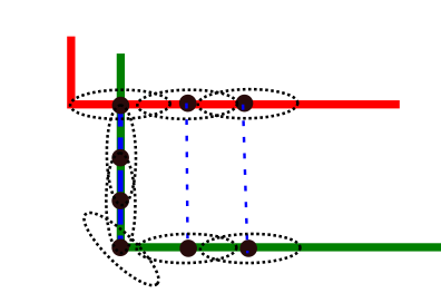
Figure 1 plane-to-plane distance
Semantic-GICP
For semantic SLAM solutions targeting AVP, semantic landmarks often exist in three-dimensional space as line features. Therefore, the assumptions made for the GICP algorithm no longer apply. The point clouds to be matched should sample from one-dimensional differential manifolds (1-manifold) in three-dimensional space, also satisfying local differentiability, with local structures of sampled points fitting into straight lines. Based on these considerations, we design and propose the Semantic-GICP (SGICP) algorithm tailored for AVP scenarios.
It is assumed that each point is sampled from a distribution characterized by significant uncertainty along one direction and smaller uncertainties along the other two directions, forming a linear distribution, namely
\[C_e= \begin{bmatrix} 1 & 0 & 0 \\ 0 & \epsilon & 0 \\ 0 & 0 & \epsilon \end{bmatrix}\]Let \(\mu_i\) and \(\nu_i\) respectively denote the local line direction vectors at points \(b_i\) and \(a_i\). \(R_\alpha\) represents the transformation that rotates the x-axis to the direction vector \(\alpha\). Therefore, \(C_i^B\) and \(C_i^A\) can also be computed as
\[\begin{aligned} &C_i^B= R_{\mu_i}C_eR_{\mu_i}^T\\ &C_i^A= R_{\nu_i}C_eR_{\nu_i}^T \end{aligned}\]In this way, the covariance matrix provides a relatively strong constraint for the error function solution in the direction perpendicular to the local straight line, while the constraint along the straight line direction is weaker. This significantly reduces erroneous associations and the impact of different geometric structures at the sampling points on the pose optimization results.
Experiments
| registration method | RPE RMSE (VO) [m] | APE RMSE (optimized) [m] |
|---|---|---|
| SGICP | 0.003545 | 0.023295 |
| SICP | 0.007652 | 0.040912 |
| ICP (PCL) | 0.008463 | 0.034878 |
| ICP_SVD | 0.006735 | 0.086893 |
| ICP_Normal (PCL) | 0.009387 | 0.043041 |
Table 1 Comparison of Accuracy for Various ICP-based Scan Matching Algorithms
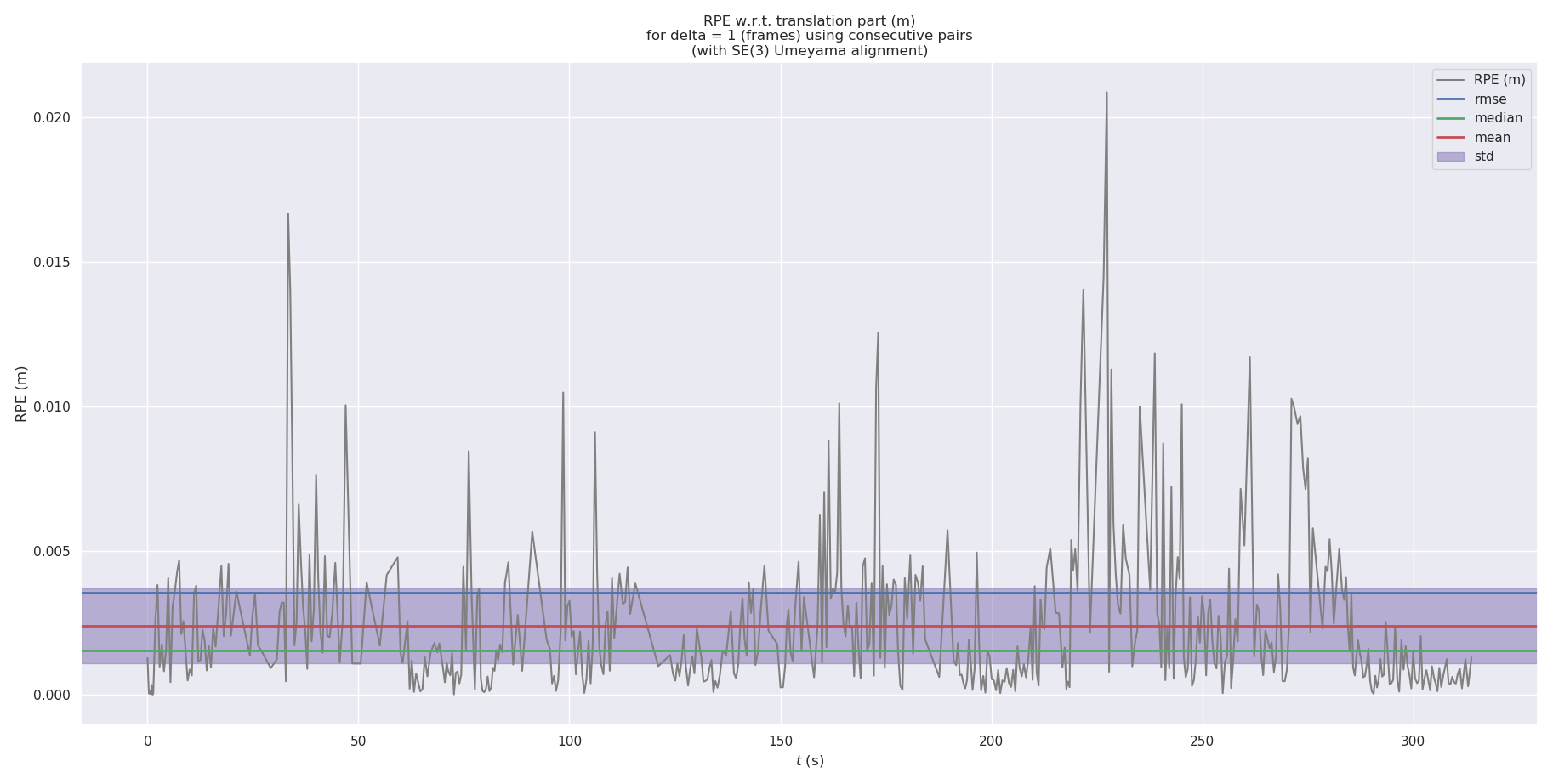
Figure 2: RPE of SGICP
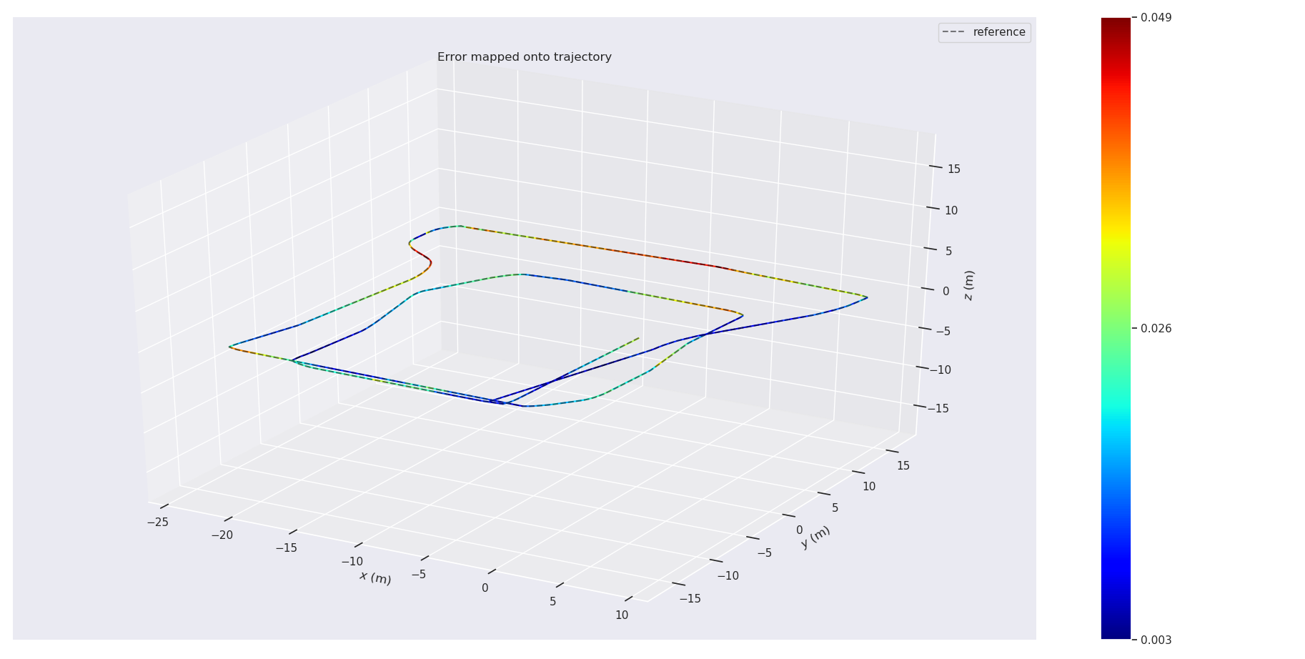
Figure 3: APE of SGICP
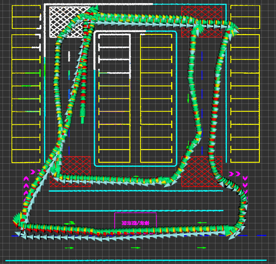
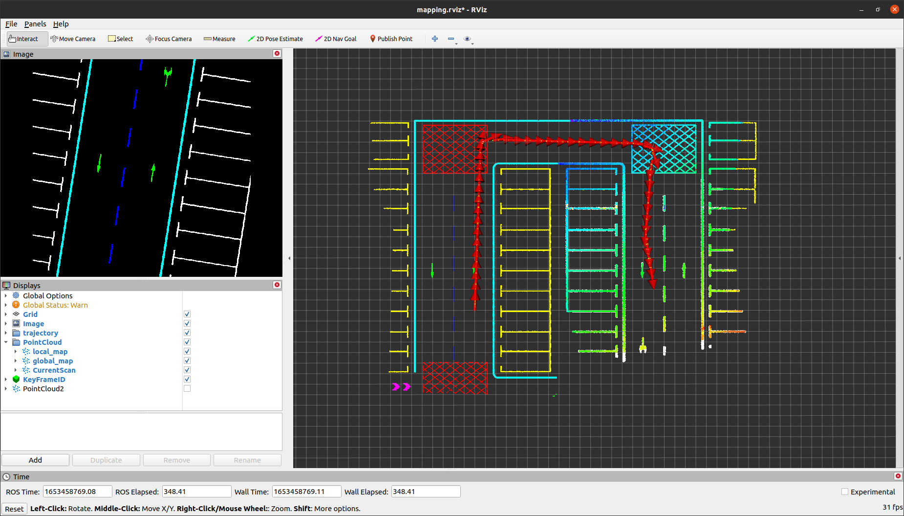
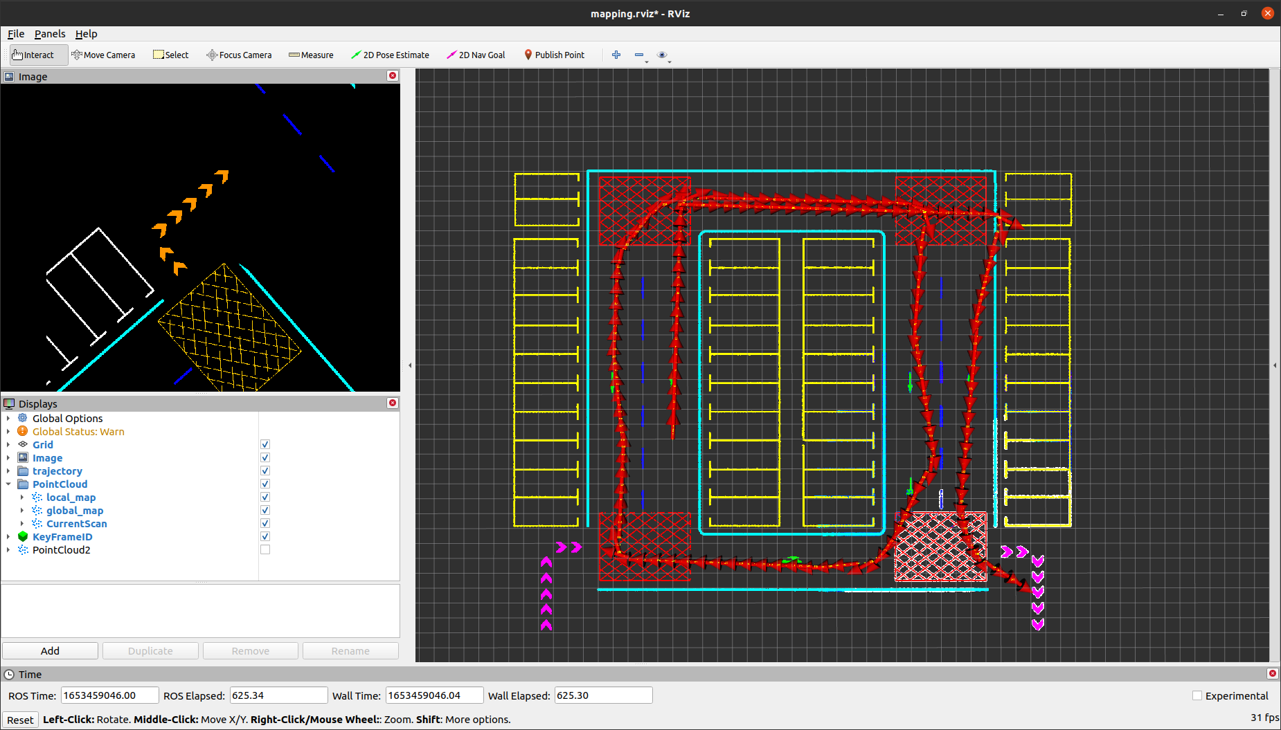
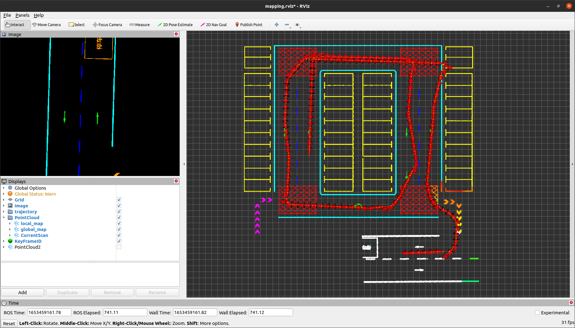
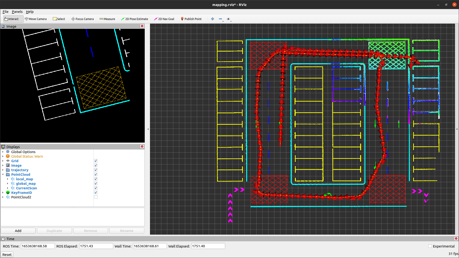
Figure 4: Mapping Results of SGICP
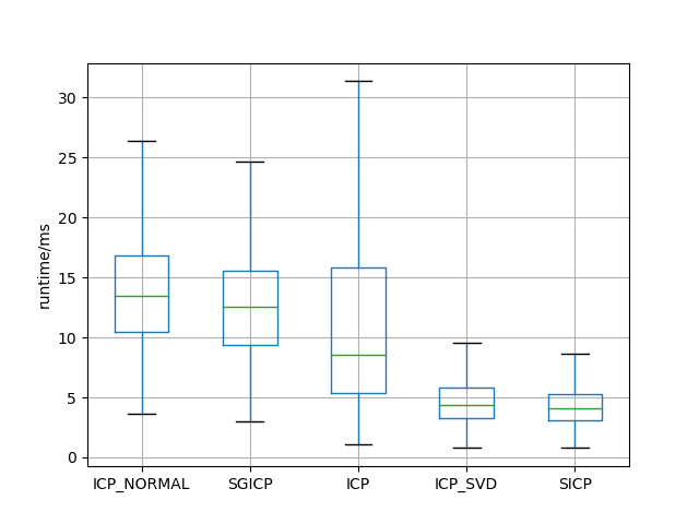
Figure 5: Comparison of Execution Time for Various ICP-based Scan Matching Algorithms
Identification and Handling of Localization Degeneration
Identification of Localization Degeneration in Visual Odometry
In visual odometry scan matching, the Hessian matrix of the objective function is calculated and then eigenvalue decomposition is performed on it.
\[\boldsymbol H= \frac{\partial^2J}{\partial\xi^2}= \boldsymbol U \boldsymbol\Lambda \boldsymbol U^T\]with \(\boldsymbol U\) and \(\boldsymbol\Lambda\) representing the eigenvectors and eigenvalues of the Hessian matrix \(\boldsymbol H\), respectively.
\[\boldsymbol U= \begin{bmatrix} \boldsymbol u_1 & \boldsymbol u_2 & \boldsymbol u_3 & \boldsymbol u_4 & \boldsymbol u_5 & \boldsymbol u_6 \end{bmatrix}\] \[\boldsymbol\Lambda= {\rm diag}\{\lambda_1,\lambda_2,\lambda_3,\lambda_4,\lambda_5,\lambda_6\}\]\(\boldsymbol u_i,i=1,\cdots,6\) represents an orthogonal basis in the six-dimensional pose space, while \(\lambda_i, i=1, \cdots, 6\) represents the constraint of the objective function \(J\) on the pose solution in the corresponding direction. When \(\lambda_i = 0\), there is a localization degeneration in the direction of \(\boldsymbol u_i\).
Hessian Matrix Calculation
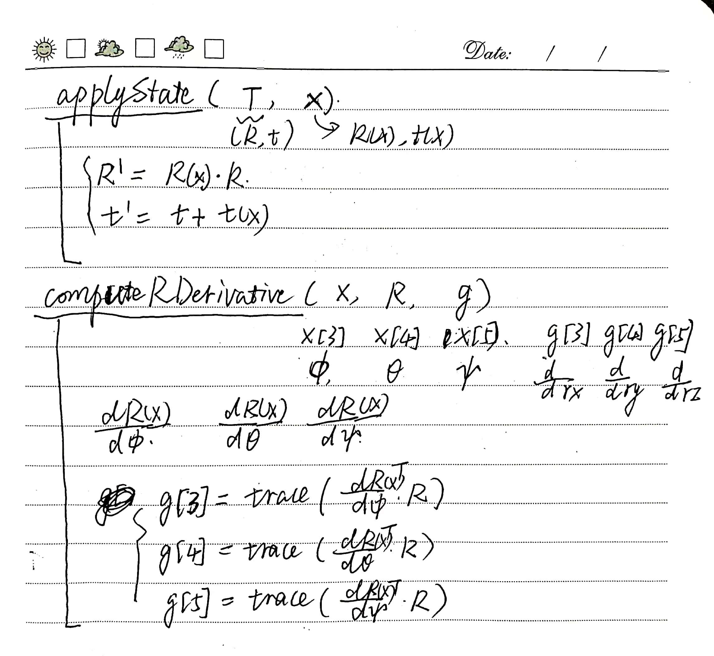
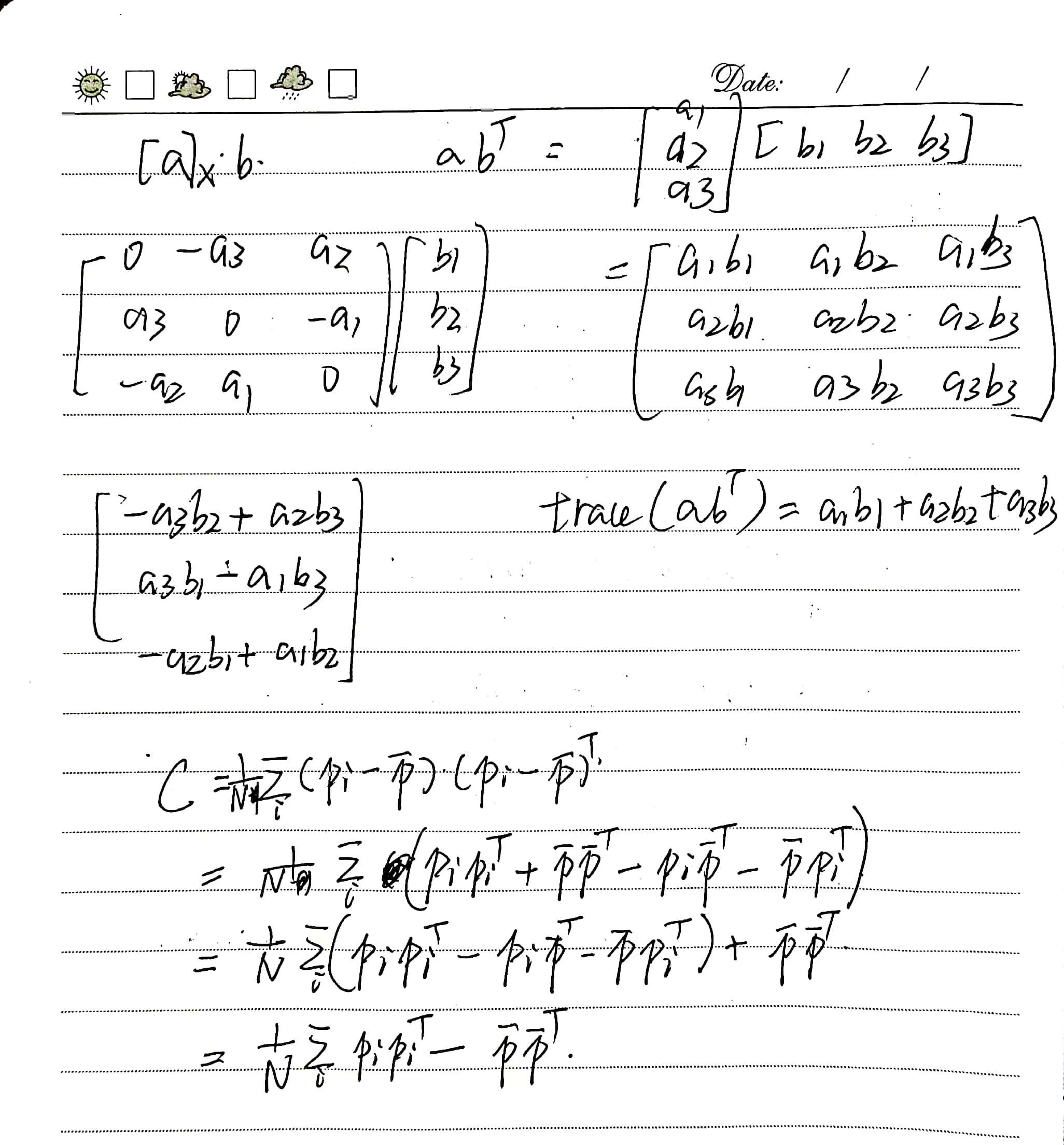
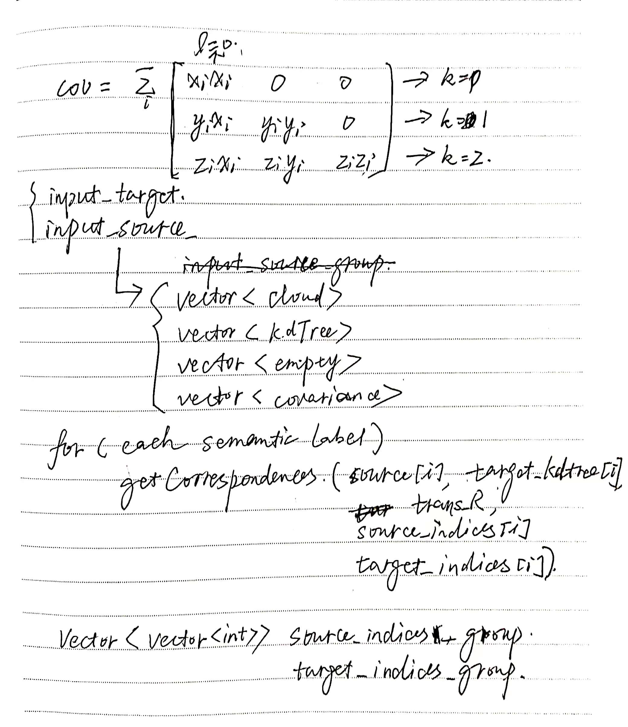
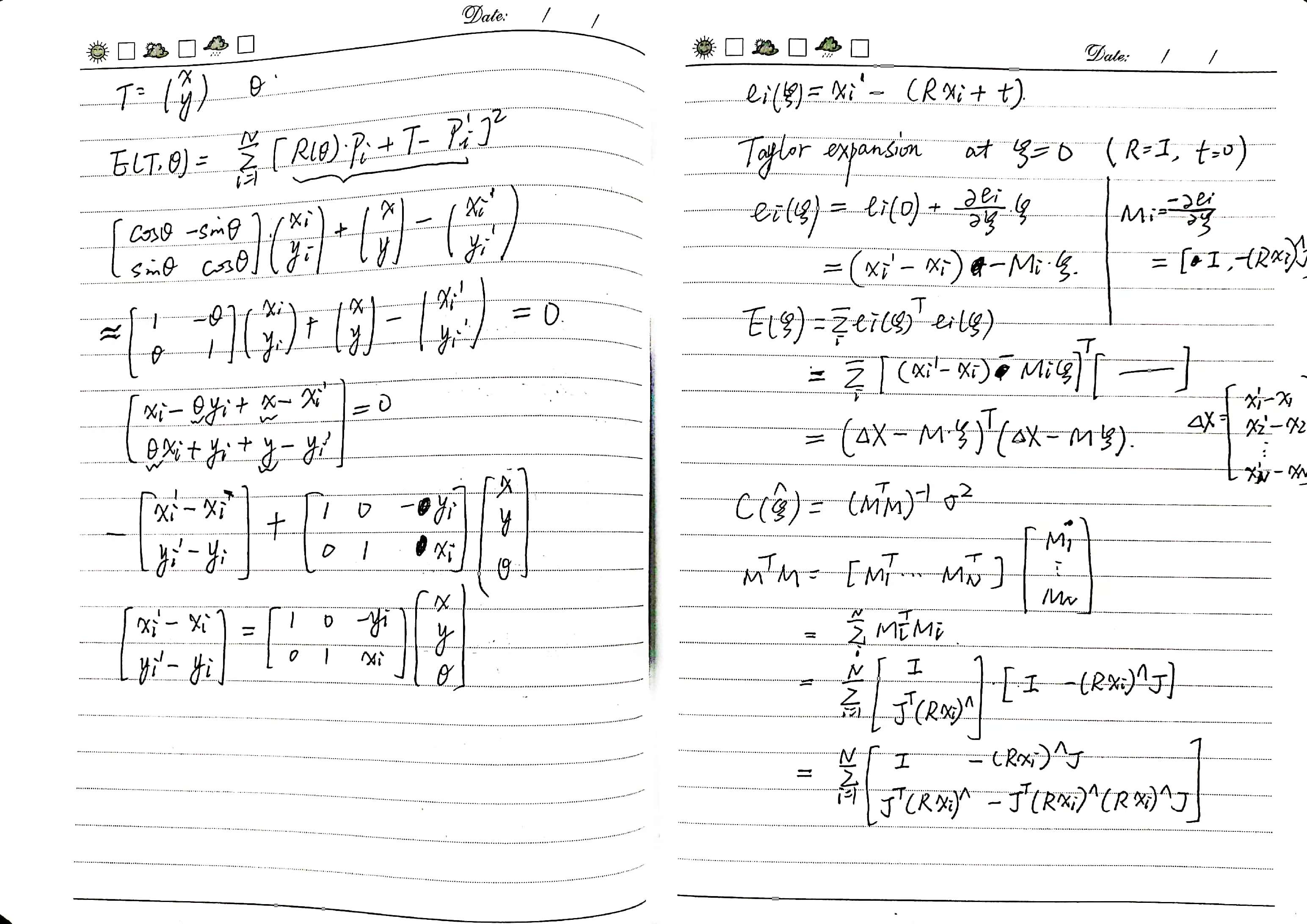
For the pose solution method in scan matching, the derivation process of the Hessian matrix of the objective function is as follows:
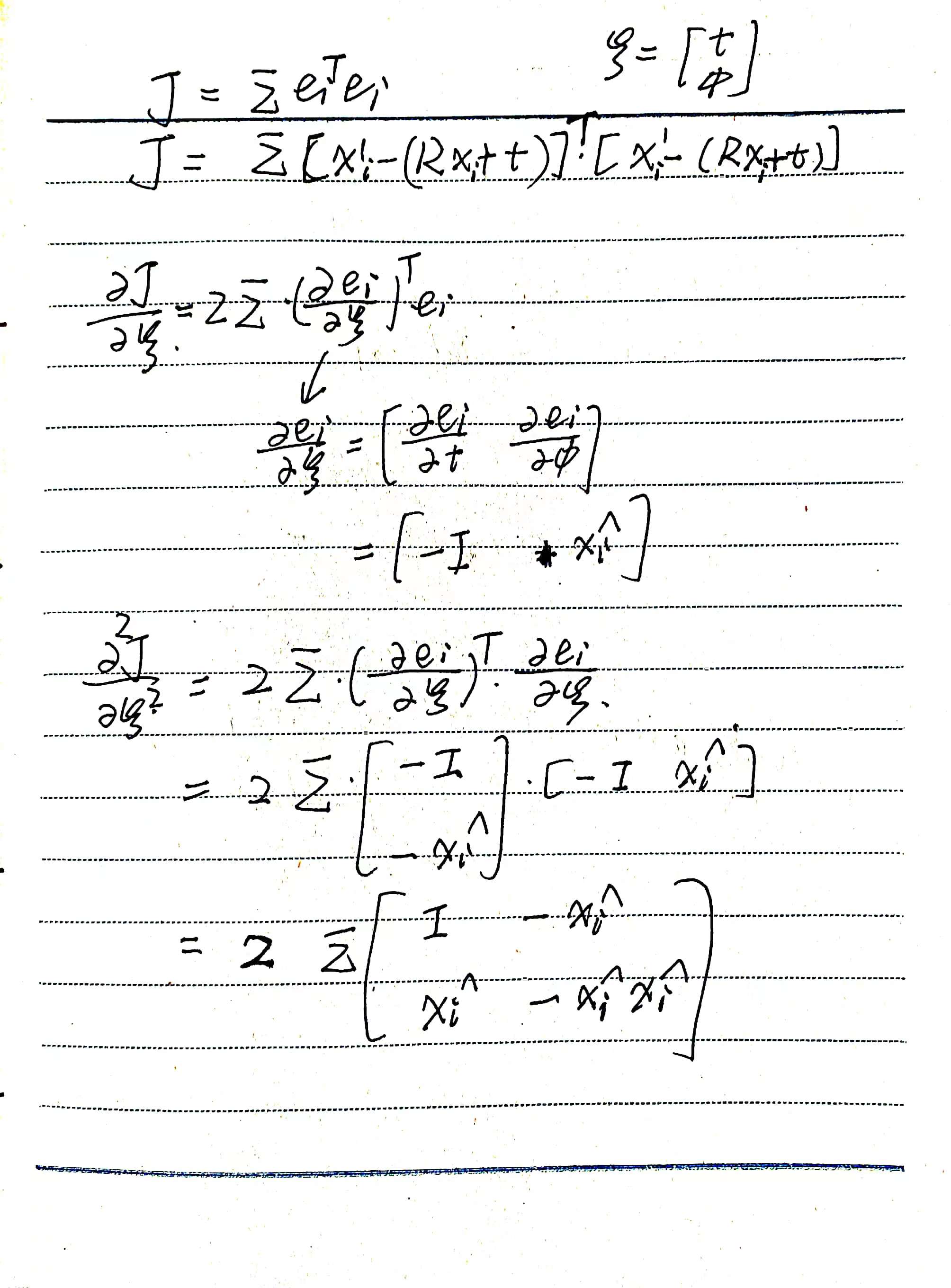
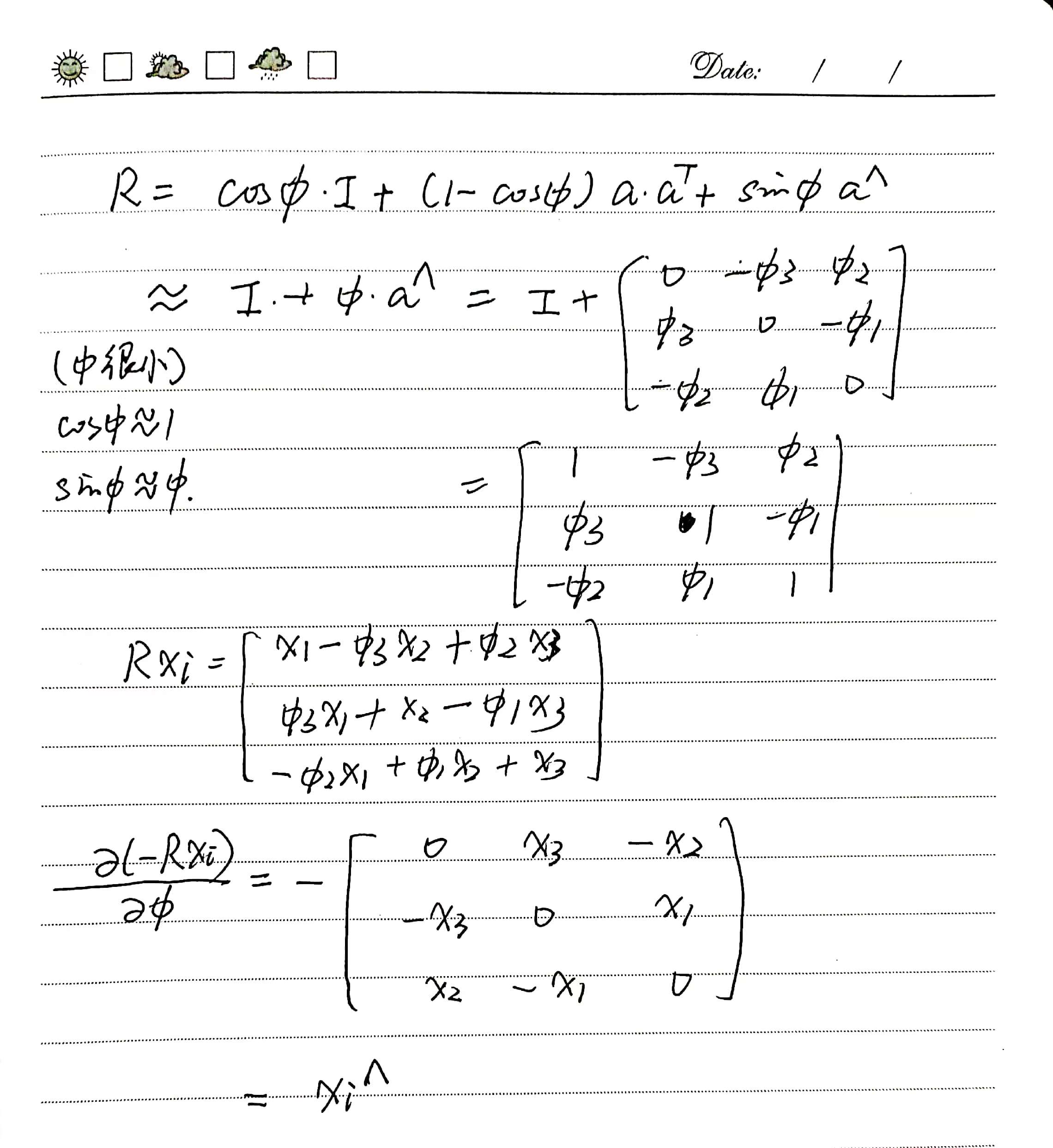
Under the assumption that the rotation angle corresponding to the rotation transformation \(\boldsymbol R\) is relatively small (this assumption is reasonable in the application scenario of inter-frame scan matching), the specific derivation process of \(\frac{\partial\boldsymbol e_i}{\partial\boldsymbol\phi}\) is shown in the following figure.
The relevant code implementation is as follows:
// models/registration/registration_interface.hpp

Eigen::Matrix<float, 6, 6> RegistrationInterface::GetCovariance()
{
  Eigen::Matrix<float, 6, 6> hessian;
  hessian.setZero();
  for (std::size_t i = 0; i < input_source_->size(); i++) {
    Eigen::Vector3f p(input_source_->at(i).x, input_source_->at(i).y, input_source_->at(i).z);
    Eigen::Matrix3f p_skew = Converter::toSkewSym(p);
    hessian.block<3, 3>(0, 0) += Eigen::Matrix3f::Identity();
    hessian.block<3, 3>(0, 3) += -p_skew;
    hessian.block<3, 3>(3, 0) += p_skew;
    hessian.block<3, 3>(3, 3) += -p_skew * p_skew;
  }
  hessian /= input_source_->size();
  Eigen::Matrix<float, 6, 6> cov = hessian.inverse() * GetFitnessScore();
  return cov;
}
Currently, the code in the RegistrationInterface interface class uses the Hessian matrix for pose covariance calculation without considering localization degeneration. The covariance calculation results are directly used in pose graph optimization based on Ceres to compute the edge weights, i.e., the information matrix, using the pseudo-inverse form of the matrix.
// models/graph_optimizer/ceres/ceres_graph_optimizer.cpp

Eigen::MatrixXd CeresGraphOptimizer::CalculateInformationMatrix(Eigen::MatrixXd cov)
{
  Eigen::SelfAdjointEigenSolver<Eigen::MatrixXd> es;
  es.compute(cov);
  Eigen::VectorXd Lambda = es.eigenvalues();
  Lambda = Lambda.cwiseAbs();
  Eigen::MatrixXd U = es.eigenvectors();
  Eigen::MatrixXd inv_Lambda = Eigen::MatrixXd::Zero(cov.rows(), cov.rows());
  for (int i = 0; i < inv_Lambda.rows(); i++) {
    if (Lambda(i) > 1e-13) {
      inv_Lambda(i, i) = 1.0 / Lambda(i);
    }
  }
  Eigen::MatrixXd info = U * inv_Lambda * U.transpose();
  return info;
}
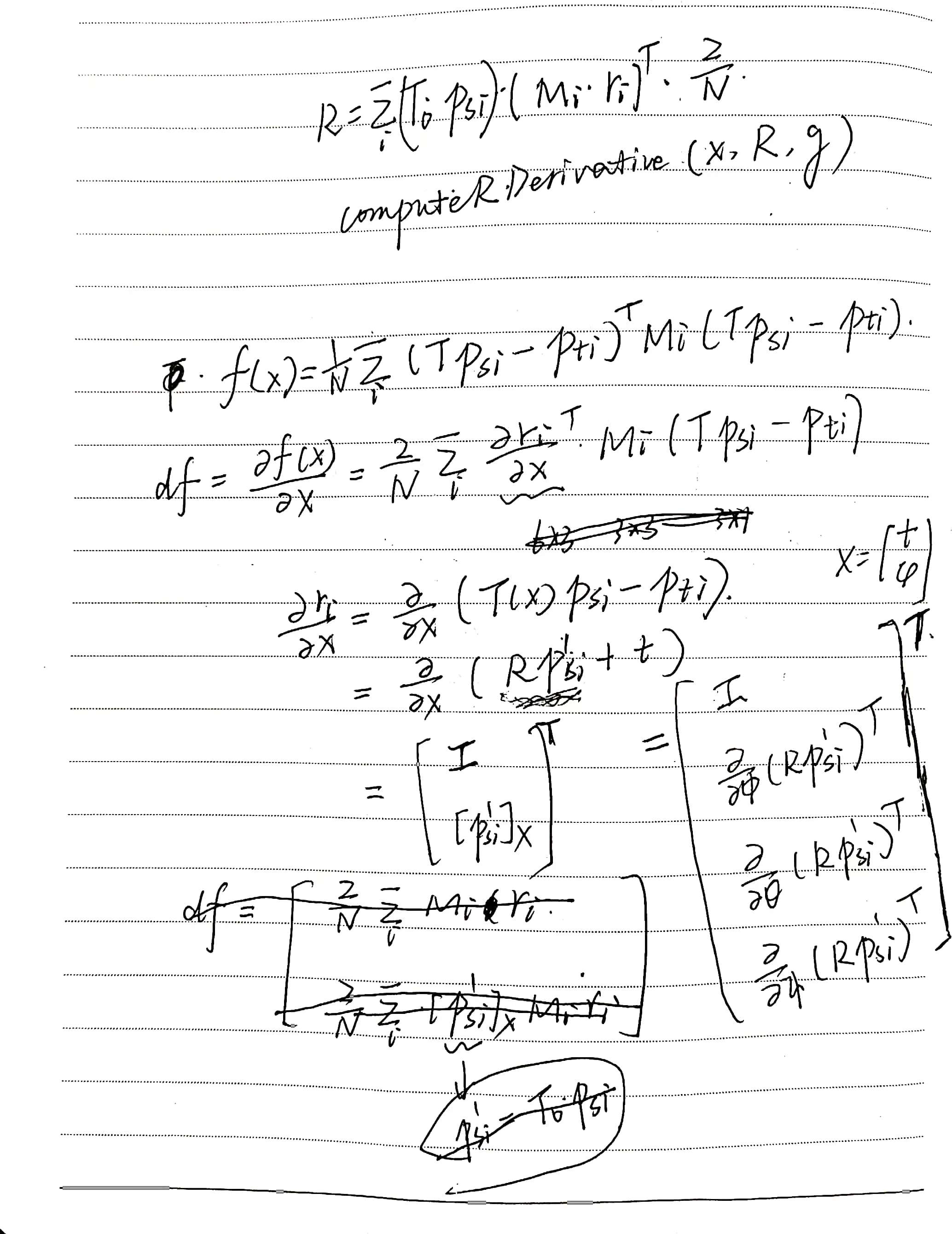
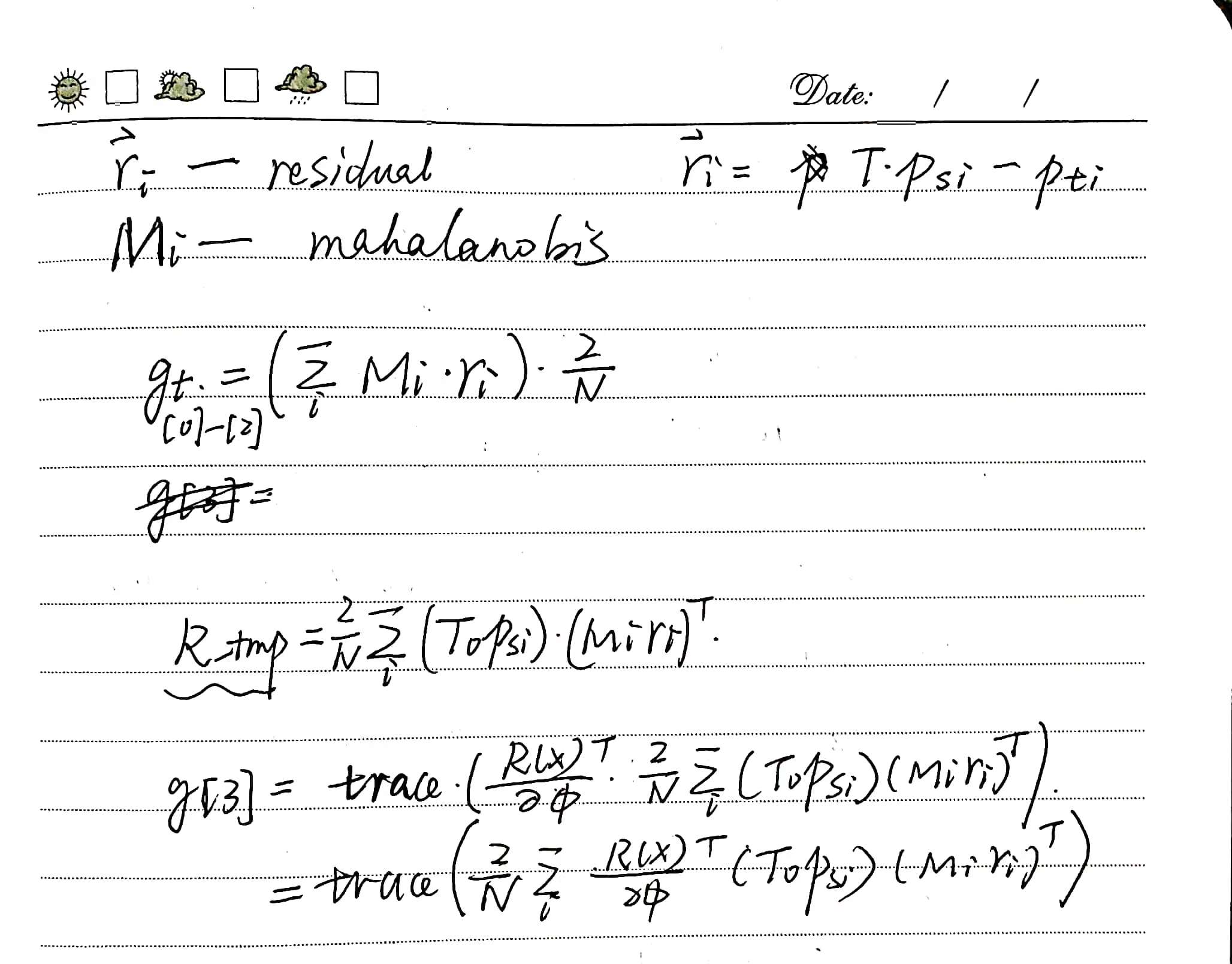
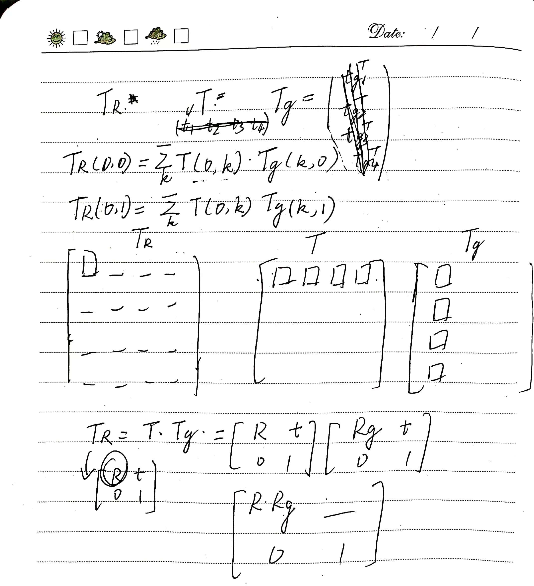
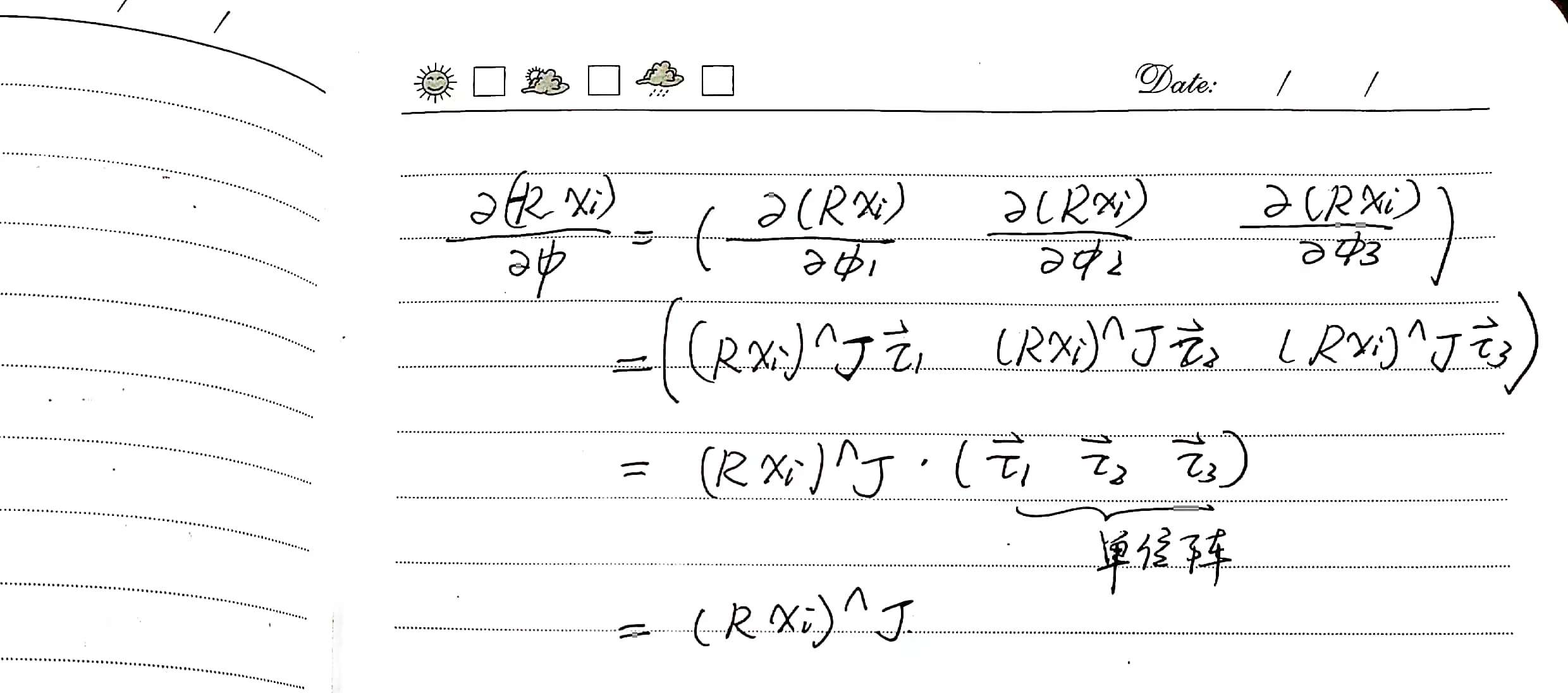
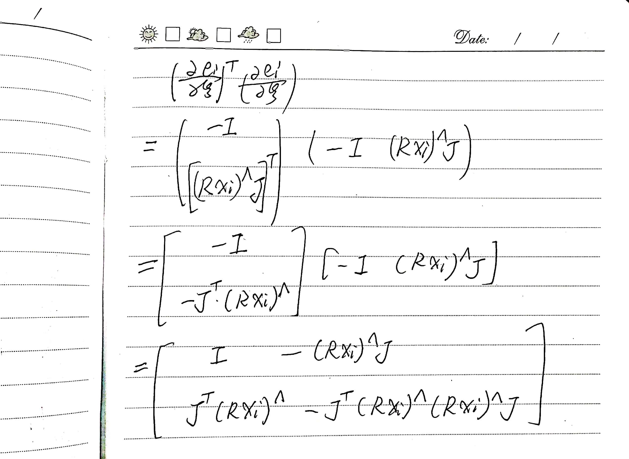
If we further consider the case of larger rotation angles, without making the assumption of small \(\phi\), so that the calculation of the Jacobian and Hessian matrices can be applicable in any situation, a more rigorous derivation is needed. The specific derivation process is shown in the following figure. Here, \(\boldsymbol J\) represents the left Jacobian of \(SO(3)\), and the specific calculation method is as follows.
\[\boldsymbol J= \frac{\sin\phi}{\phi}\boldsymbol I+ \left(1-\frac{\sin\phi}{\phi}\right)\boldsymbol a\boldsymbol a^T+ \frac{1-\cos\phi}{\phi}\boldsymbol a^\wedge \\\]其中
\[\phi=|\boldsymbol\phi|, \quad \boldsymbol a=\frac{\phi}{|\phi|}\]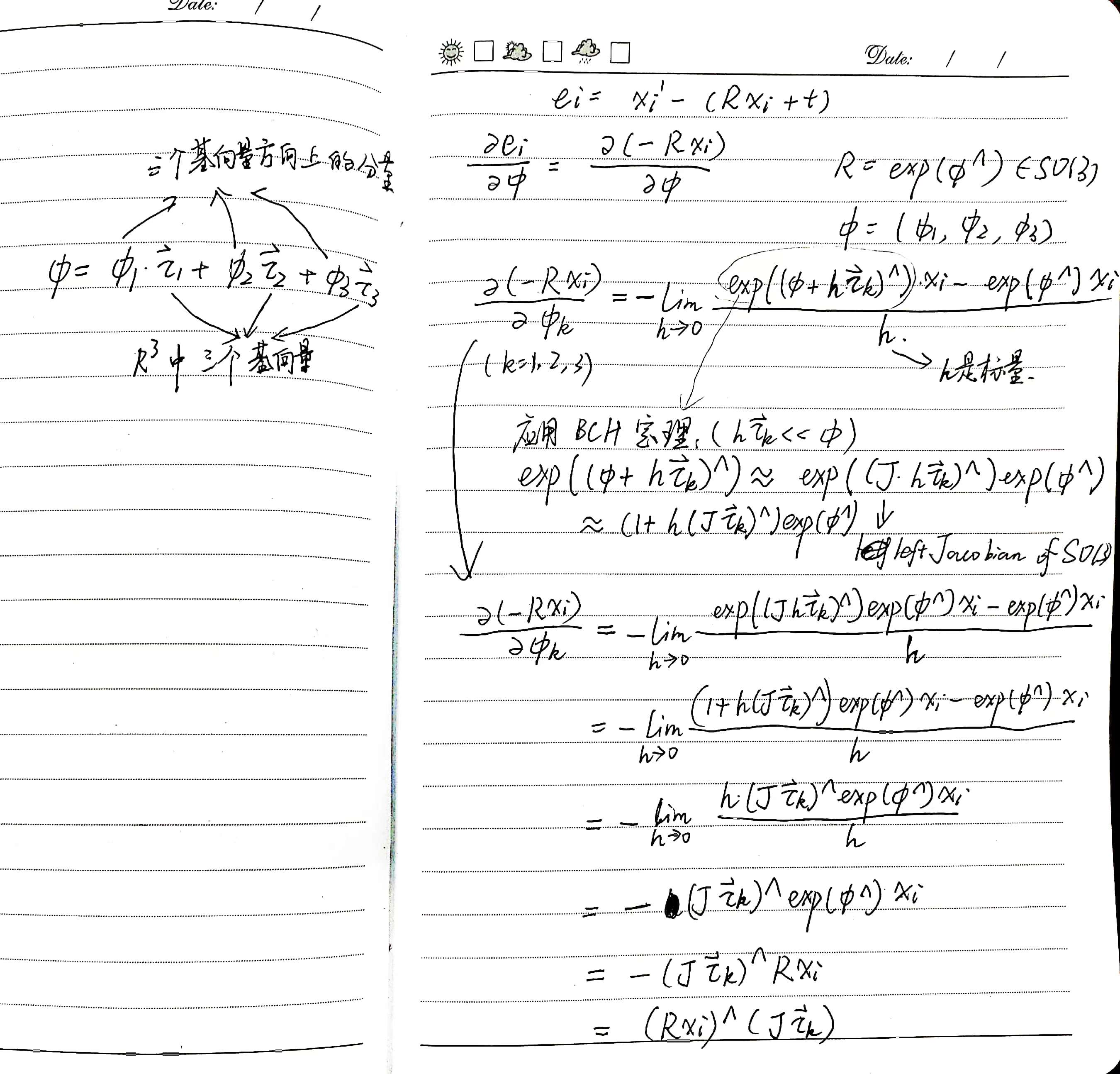
Numerical Differences in the Hessian Matrix Caused by Observation Data Coordinates
Read the literature: Bengtsson O, Baerveldt A J. Robot localization based on scan-matching - estimating the covariance matrix for the IDC algorithm [J]. Robotics & Autonomous Systems, 2003, 44(1): 29-40.
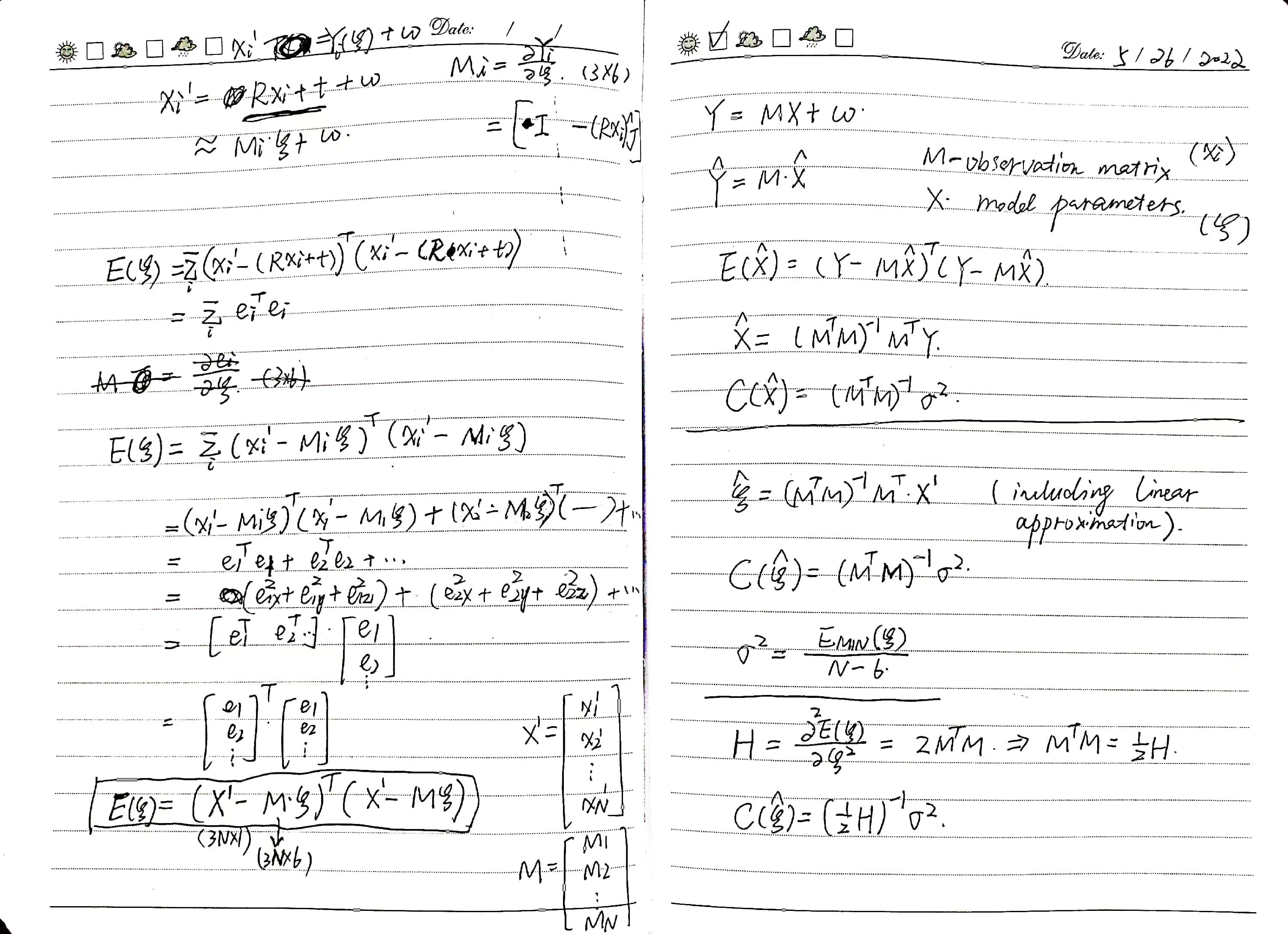
When using linear least squares for parameter identification, the unbiased estimate of parameter uncertainty is
\[\boldsymbol C(\hat{\boldsymbol\xi})= (\boldsymbol M^T\boldsymbol M)^{-1}\sigma^2\]where \(\sigma^2\) is the variance of the noise, it can also be unbiasedly estimated during the solving process.
\[\hat{\sigma}^2= \frac{E(\hat{\boldsymbol\xi})} {N-6}\]It can be seen that the uncertainty estimation of parameters is mainly determined by three factors: the numerical values of observation data, the objective function values at the optimal estimate, and the amount of observation data. In the context of scan matching, the observation matrix \(\boldsymbol M\) contains only the coordinate information of points transformed by the objective function (due to linearization of the rotation vector \(\boldsymbol\phi\), where the rotation transformation affects only the transformed point cloud).
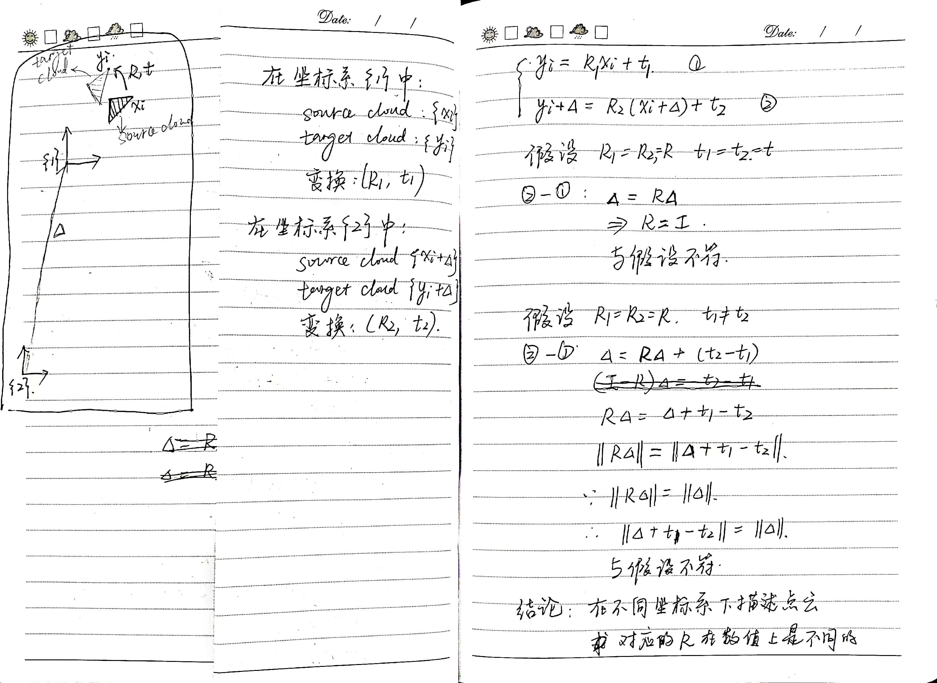
Next, considering whether the rotational transformation for registering point clouds remains consistent numerically when represented in different coordinate systems. Through simple analysis (see figure below), it is evident that at least in different coordinate systems with only translation transformations, the numerical values of their respective registration transformations are inconsistent.
Identification and Handling of Localization Degeneration
In the GetCovariance function of the scan matching interface class, the calculation of the Hessian matrix has been modified to remove assumptions about the size of rotation angles, making it applicable in any scenario.
The Hessian matrix is decomposed into eigenvalues and eigenvectors. The six eigenvectors span the six-dimensional pose space, and the corresponding eigenvalues represent the strength of constraints in each direction. When an eigenvalue in a specific direction is zero (or very small), it indicates localization degeneration in that direction.
In contrast to the previous development stage where hessian.inverse() was used to invert the Hessian matrix, in this stage, each eigenvalue direction is processed. For directions where localization degeneration occurs, the variance in that direction is set to zero in the covariance calculation. Similarly, when adding edges in Ceres graph optimization with covariance matrix eigenvalues of zero, the corresponding information value in the information matrix calculation is set to zero. This ensures that during graph optimization, residuals from degenerate directions do not affect the optimization variables.
// models/registration/registration_interface.cpp

Eigen::Matrix<float, 6, 6> RegistrationInterface::GetCovariance()
{
  Eigen::Matrix3f R = cloud_pose_.linear();
  Eigen::Vector3f phi = Converter::Log(R);
  Eigen::Matrix3f J = ComputeJacobianSO3(phi);

  // computation of hessian matrix;
  Eigen::Matrix<float, 6, 6> hessian;
  hessian.setZero();
  for (std::size_t i = 0; i < input_source_->size(); i++) {
    Eigen::Vector3f p(input_source_->at(i).x, input_source_->at(i).y, input_source_->at(i).z);
    Eigen::Matrix3f Rp_skew = Converter::toSkewSym(R * p);
    hessian.block<3, 3>(0, 0) += Eigen::Matrix3f::Identity();
    hessian.block<3, 3>(0, 3) += -Rp_skew * J;
    hessian.block<3, 3>(3, 0) += J.transpose() * Rp_skew;
    hessian.block<3, 3>(3, 3) += -J.transpose() * Rp_skew * Rp_skew * J;
  }
  hessian /= input_source_->size();

  // psedo-inverse of hessian;
  // identify the degeneration;
  Eigen::SelfAdjointEigenSolver<Eigen::Matrix<float, 6, 6>> es;
  es.compute(hessian);
  Eigen::Matrix<float, 6, 1> eigenvalues = es.eigenvalues().cwiseAbs();
  Eigen::Matrix<float, 6, 6> eigenvectors = es.eigenvectors();
  Eigen::Matrix<float, 6, 6> eigenvalues_inv = Eigen::Matrix<float, 6, 6>::Zero();
  for (int i = 0; i < 6; i++) {
    if (eigenvalues(i) > 1e-7) {
      eigenvalues_inv(i, i) = 1.0 / eigenvalues(i);
    }
  }
  Eigen::Matrix<float, 6, 6> hessian_inv = eigenvectors * eigenvalues_inv * eigenvectors.transpose();

  Eigen::Matrix<float, 6, 6> cov = hessian_inv * GetFitnessScore();

  return cov;
}
Eigen::Matrix3f RegistrationInterface::ComputeJacobianSO3(const Eigen::Vector3f &phi)
{
  float phy = phi.norm();
  if (phy < 1e-7)
    return Eigen::Matrix3f::Identity();
  else {
    Eigen::Vector3f a = phi / phy;
    return Eigen::Matrix3f::Identity() * sin(phy) / phy + a * a.transpose() * (1 - sin(phy) / phy) +
           Converter::toSkewSym(a) * (1 - cos(phy)) / phy;
  }
}
[registration] eigenvalues = 0.989348 0.993552 0.999998  16.0163  23.1255  39.1119
[registration] eigenvectors =
    0.175787      0.83729    -0.517577  -0.00691053     -0.00154    0.0103471
    0.160605    -0.543076    -0.824139   0.00221123   -0.0047209  -0.00649815
     0.97098   -0.0617677     0.230019  -0.00762599   -0.0203846 -2.94937e-06
  -0.0172826   0.00442972 -1.11965e-06     0.307042    -0.951527  -0.00144674
   0.0142625   0.00544714  5.02623e-08     0.951635     0.306846   -0.0018499
 0.000771046    0.0121771 -8.35513e-07  -0.00229072  0.000823814    -0.999923
[registration] eigenvalues =  0.99732 0.998226 0.999998  20.8495  25.4666  46.2896
[registration] eigenvectors =
  -0.0292447    -0.998948   -0.0345322   -0.0054239 -0.000870817   0.00508309
    0.432673    0.0184886     -0.90135   0.00107524  -0.00440993 -0.000194337
   -0.901015    0.0413031    -0.431713  -0.00181522   0.00929514 -1.31404e-07
  -0.0105017  0.000108864 -8.05822e-06     0.194108    -0.980924 -4.25527e-06
-0.000225524  -0.00549407 -2.96679e-07     0.980962     0.194117   -0.0010237
 0.000232297   0.00507578   3.1432e-07   0.00103292  0.000198134     0.999986
[registration] eigenvalues = 0.500933 0.709362        1  15.3146  22.2708   37.364
[registration] eigenvectors =
  -0.0335301     0.117831    -0.992398   0.00120082  -0.00503306    0.0105361
  0.00131298     0.989025     0.118326   0.00369037  0.000745354    0.0883873
    0.987821   0.00270144   -0.0338427   -0.0223112     0.150199  6.81956e-05
  -0.0108242  -0.00527782 -1.53668e-08     0.976117     0.216273    0.0166375
   -0.151548  0.000386434  1.62661e-07      -0.2154     0.964694  -0.00121469
-0.000166557    0.0889363  9.39908e-08    0.0169086   0.00245959    -0.995891
[registration] eigenvalues =  0.81157 0.922223        1  10.7131  24.3138  34.8954
[registration] eigenvectors =
  -0.0296467     0.577013    -0.815721   0.00219719  -0.00417403    0.0274864
  -0.0746723    -0.814124    -0.574455    0.0103402  2.71433e-05    -0.039003
   -0.988912    0.0442767    0.0678315     0.113994   -0.0499667  0.000232017
    0.105782   0.00312969 -7.30797e-08     0.982783      0.15128  -0.00719585
  -0.0663682   0.00480734  5.81408e-08    -0.144904     0.987144   -0.0110124
  0.00184005    0.0476064 -1.66578e-08   -0.0057998   -0.0121017    -0.998774
Degradation Scene Testing and Problem Analysis
Since there are no degradation scenes in the simulation data, in the semantic point reconstruction part of the code, filter out point clouds with a single semantic label (add line 10, filter semantic points with label 5, specifically semantic points on the lane centerline), manually generating localization degradation scenarios.
  // data_pretreat/data_pretreat_flow.cpp

  for (int u = 0; u < img_height; u++) {
    for (int v = 0; v < img_width; v++) {
      rgb[0] = current_vision_data_.image[u * img_width * 3 + v * 3 + 2];
      rgb[1] = current_vision_data_.image[u * img_width * 3 + v * 3 + 1];
      rgb[2] = current_vision_data_.image[u * img_width * 3 + v * 3 + 0];
      std::map<unsigned long, unsigned char>::iterator it = semantic_label_map_.find(RGB2Key(rgb));
      if (it != semantic_label_map_.end()) {
        if (it->second != 5) continue;
        // semantic landmark pixels;
        current_cloud_data_.cloud_ptr->push_back(Pixel2Point(u, v, it->second, px_width, cx));
        mark[u][v] = 255;
      }
    }
  }
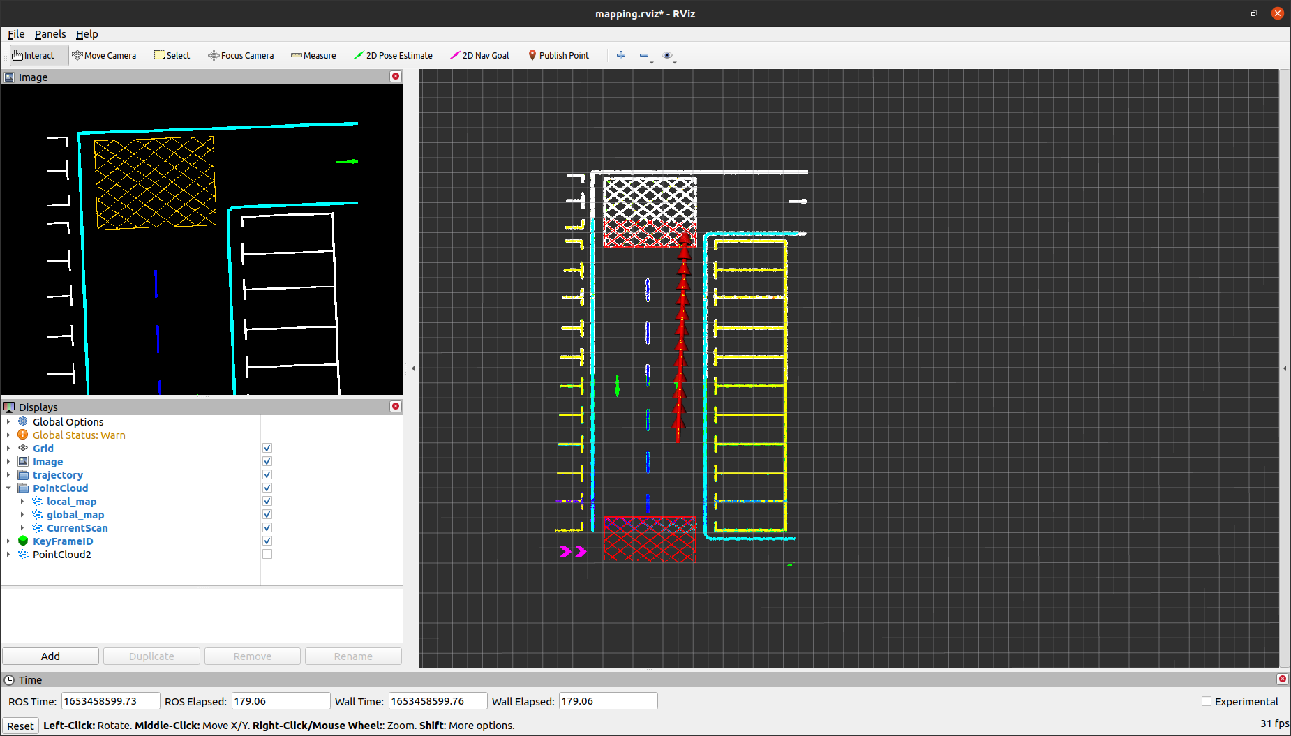
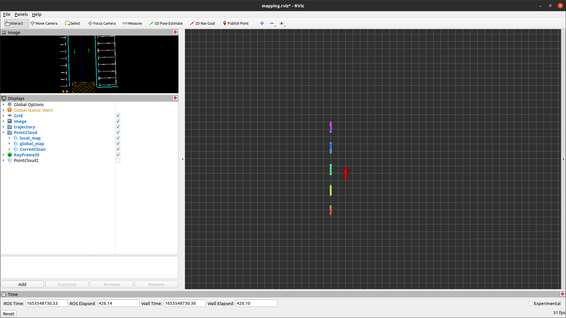
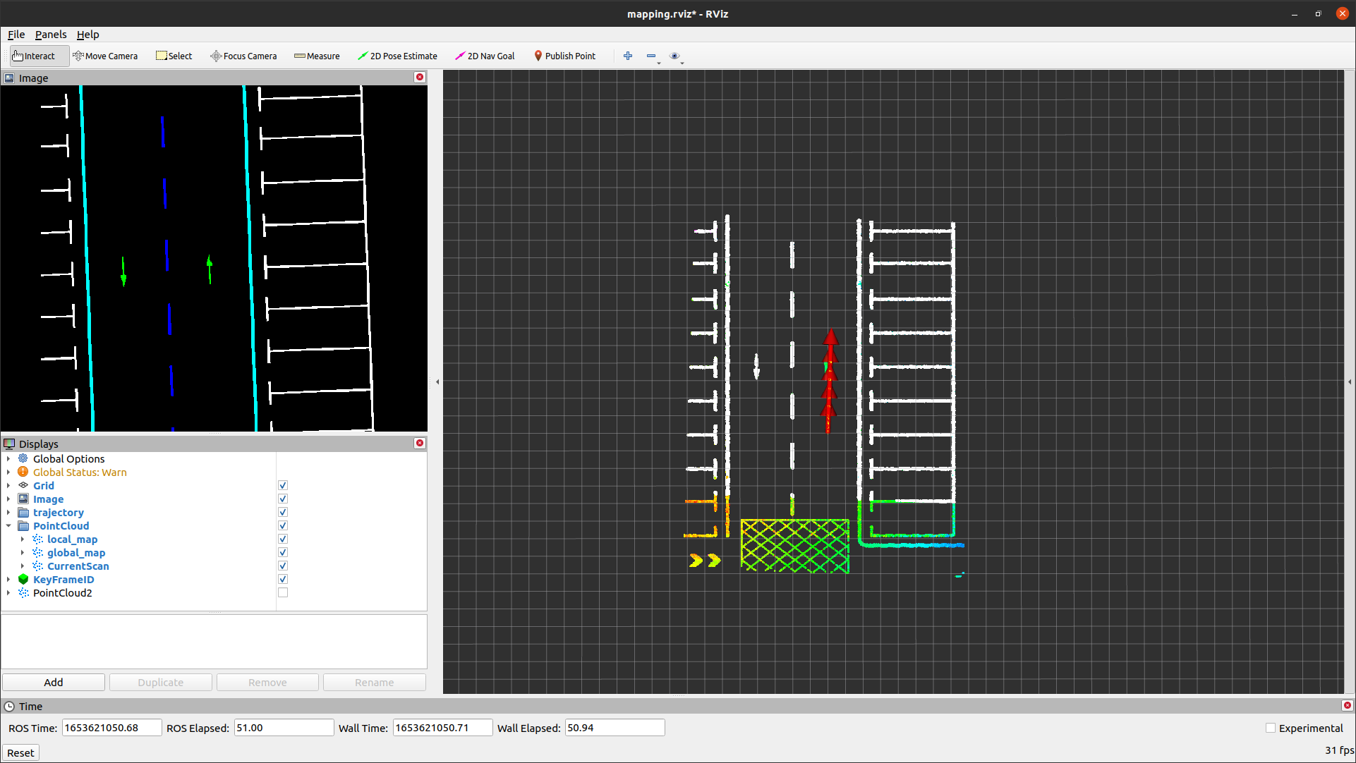
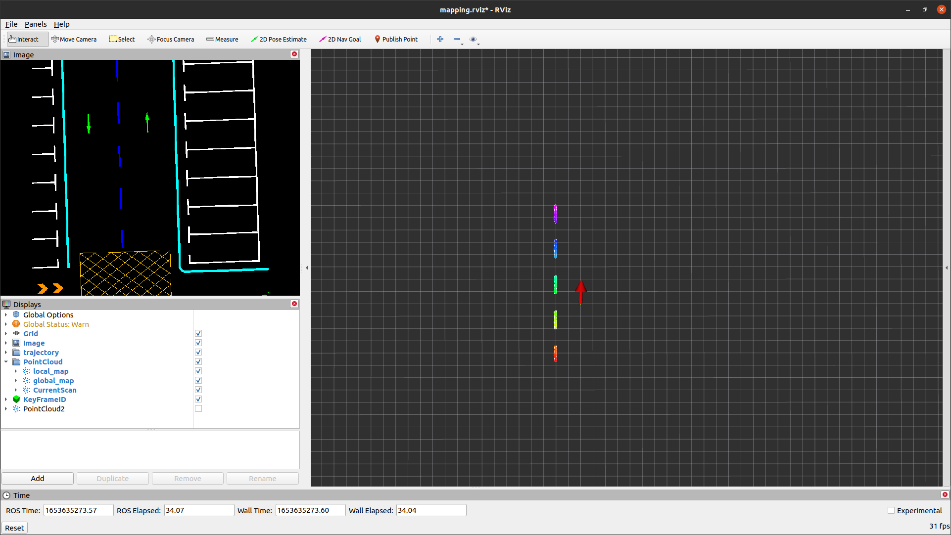
The running results and corresponding semantic point clouds are as follows.
[registration] eigenvalues = 0.000247547 0.676283  1  4.10213  20.2055 23.6316
[registration] eigenvectors =
  0.00141902     0.769248    -0.632291  0.000670215  -0.00017796    0.0920006
  -0.0482712    -0.626846    -0.773666   -0.0227798   0.00612038   -0.0749701
    -0.89717    0.0349437    0.0406262    -0.423379     0.113786    0.0041774
    0.438843 -0.000190148  -7.9749e-08    -0.859574     0.261814   0.00158868
   0.0130772   0.00638164  6.89979e-08      -0.2849    -0.956962   -0.0533357
 1.33349e-06      0.11858  2.30429e-07    0.0139493     0.051898    -0.991489
From the running results, it can be observed that there is degradation in one dimension, but the direction of this dimension deviates from the expected.
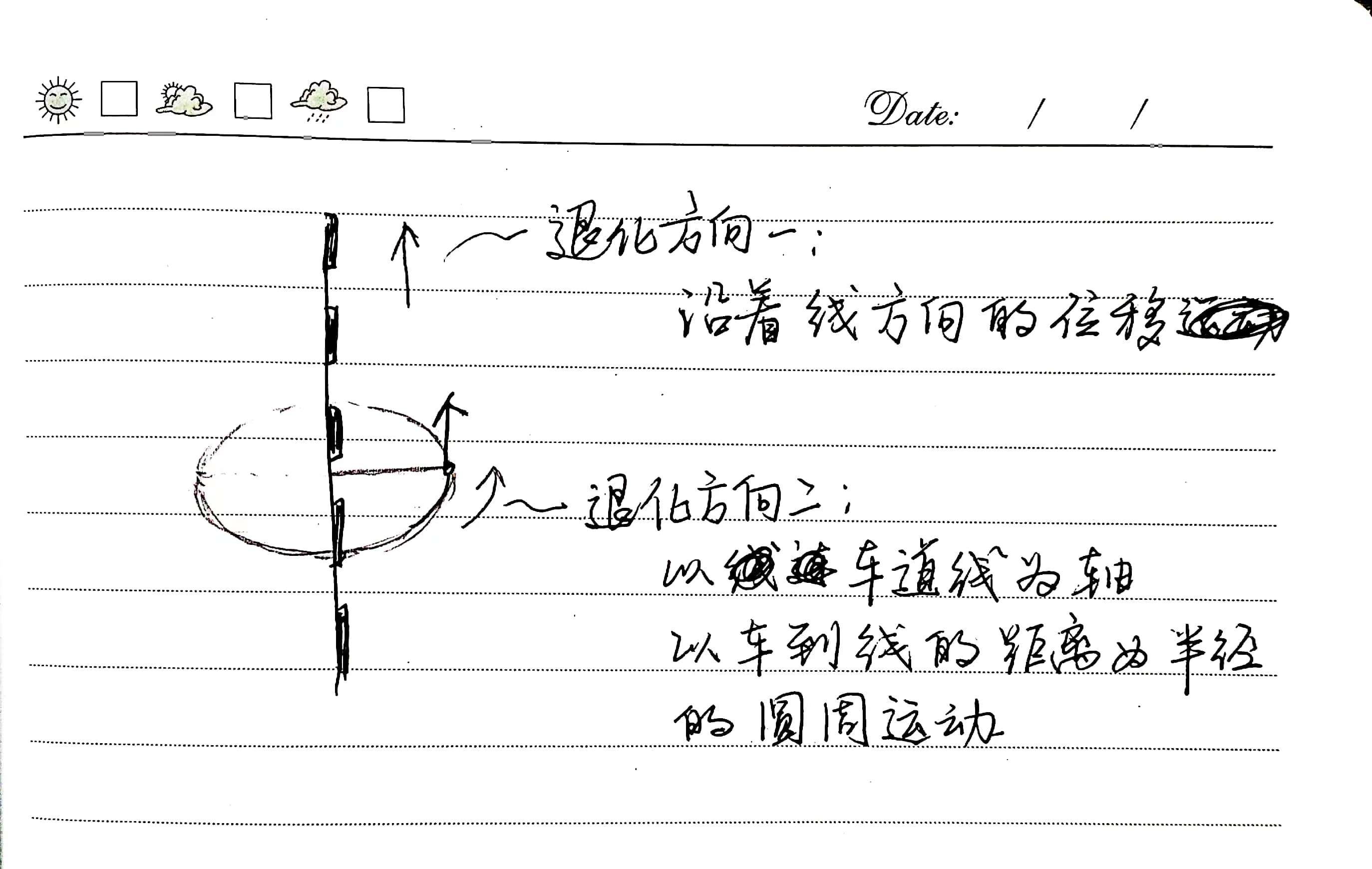
For three-dimensional scan data distributed linearly in space, theoretically, there should be two degradation directions (as shown in the figure below): one is along the direction of the line’s displacement, and the other is rotational movement around the line with the distance from the line to the origin as the radius. Since this project mainly focuses on the movement of the vehicle in three-dimensional space on the map, the first type of degradation is more worthy of our attention.
However, in the above-displayed running results, it unexpectedly shows the direction of the second type of degradation.
The analysis reveals that the objective function is defined for point-to-point matching, and given the known correspondences, degradation in the direction depicted in the previous figure does not occur.
Based on the above analysis, for different types of ICP algorithms, adjustments are made to the form of the objective function used to solve the Hessian matrix. Taking SGICP as an example, in the registration_interface interface class, the information matrix terms in the objective function are retained. When calculating the Hessian matrix, these terms are taken into account. This reduces the constraint strength of the residual terms on motion along the lane direction, thereby identifying degradation along the lane direction.
The code modification is as follows, primarily incorporating the calculation of the Hessian matrix with informations_ stored in the interface class, particularly lines 14-17.
// models/registration/registration_interface.cpp

Eigen::Matrix<float, 6, 6> RegistrationInterface::GetCovariance()
{
  Eigen::Matrix3f R = cloud_pose_.linear();
  Eigen::Vector3f phi = Converter::Log(R);
  Eigen::Matrix3f J = ComputeJacobianSO3(phi);

  Eigen::Matrix<float, 6, 6> hessian;
  hessian.setZero();
  for (std::size_t i = 0; i < input_source_->size(); i++) {
    Eigen::Vector3f p(input_source_->at(i).x, input_source_->at(i).y, input_source_->at(i).z);
    Eigen::Matrix3f Rp_skew = Converter::toSkewSym(R * p);
    hessian.block<3, 3>(0, 0) += informations_[i];
    hessian.block<3, 3>(0, 3) += -informations_[i] * Rp_skew * J;
    hessian.block<3, 3>(3, 0) += J.transpose() * Rp_skew * informations_[i];
    hessian.block<3, 3>(3, 3) += -J.transpose() * Rp_skew * informations_[i] * Rp_skew * J;
  }
  hessian /= input_source_->size();

  Eigen::SelfAdjointEigenSolver<Eigen::Matrix<float, 6, 6>> es;
  es.compute(hessian);
  Eigen::Matrix<float, 6, 1> eigenvalues = es.eigenvalues().cwiseAbs();
  Eigen::Matrix<float, 6, 6> eigenvectors = es.eigenvectors();
  Eigen::Matrix<float, 6, 6> eigenvalues_inv = Eigen::Matrix<float, 6, 6>::Zero();
  for (int i = 0; i < 6; i++) {
    if (eigenvalues(i) > 1e-7) {
      eigenvalues_inv(i, i) = 1.0 / eigenvalues(i);
    }
  }
  Eigen::Matrix<float, 6, 6> hessian_inv = eigenvectors * eigenvalues_inv * eigenvectors.transpose();

  Eigen::Matrix<float, 6, 6> cov = hessian_inv * GetFitnessScore();

  return cov;
}

// models/registration/sgicp_registration.cpp
// SGICPRegistration::ScanMatch
  cloud_pose_ = result_pose;
  input_source_.reset(new CloudData::CLOUD());
  informations_.resize(0);
  for (std::size_t i = 0; i < SEMANTIC_NUMS; i++) {
    for (std::size_t j = 0; j < source_indices_group[i].size(); j++) {
      std::size_t idx = source_indices_group[i][j];
      input_source_->push_back(input_source_group_[i]->at(idx));
      informations_.push_back(group_informations_[i][idx]);
    }
  }
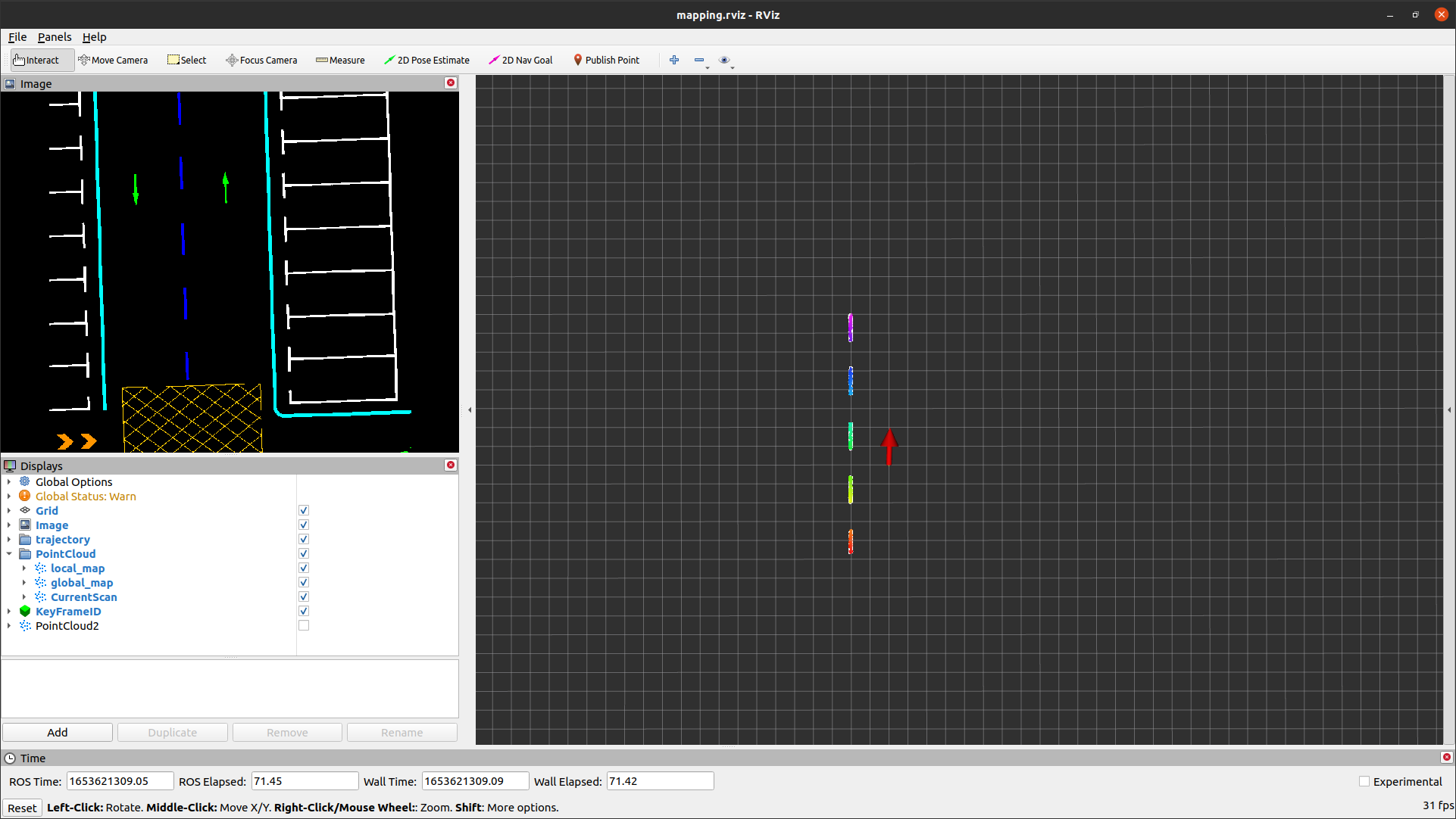
The modified running results are shown below, where two degradation directions can be observed: rotational movement around the lane centerline and translational movement along the lane centerline direction.
[registration] eigenvalues = 0.123623 0.935589  173.807  2041.44  4730.2  10028.3
[registration] eigenvectors =
  0.00131299     0.999372   -0.0353092  0.000280167  -0.00273564 -1.18781e-05
  -0.0481662    0.0354307     0.993402  -0.00717455    0.0976024  0.000664447
    -0.89737 -0.000350337   -0.0468704    -0.423313   0.00242729     0.115456
    0.438455  0.000181967    0.0133516    -0.858807    0.0154893     0.264176
   0.0127312  1.84039e-05  -0.00151271    -0.287942   0.00702575    -0.957536
 2.14243e-06 -0.000729898   -0.0976181    0.0171383     0.995074   0.00230166
Since this project mainly focuses on the two-dimensional spatial movement of the vehicle on the ground plane, it is unnecessary to detect all degradation scenarios in three-dimensional space. For example, the second degradation direction mentioned earlier, which involves rotational movement around the lane direction, is not feasible in reality for vehicle motion and therefore is not within the scope of this project’s considerations.
Extraction of Two-Dimensional Pose Subspace from Six-Dimensional Pose Space
When determining localization degradation, it is necessary to extract the three-dimensional pose subspace required for two-dimensional plane motion from the six-dimensional pose space. Define the selection matrix \(\boldsymbol S\) as
\[\boldsymbol S= \begin{bmatrix} 1 & 0 & 0 & 0 & 0 & 0 \\ 0 & 1 & 0 & 0 & 0 & 0 \\ 0 & 0 & 0 & 0 & 0 & 1 \\ \end{bmatrix}\]Then, the two-dimensional plane pose (\boldsymbol{\zeta}) corresponding to the three-dimensional pose (\boldsymbol{\xi}) in the pose space can be computed as
\[\boldsymbol\zeta=\boldsymbol S\boldsymbol\xi\]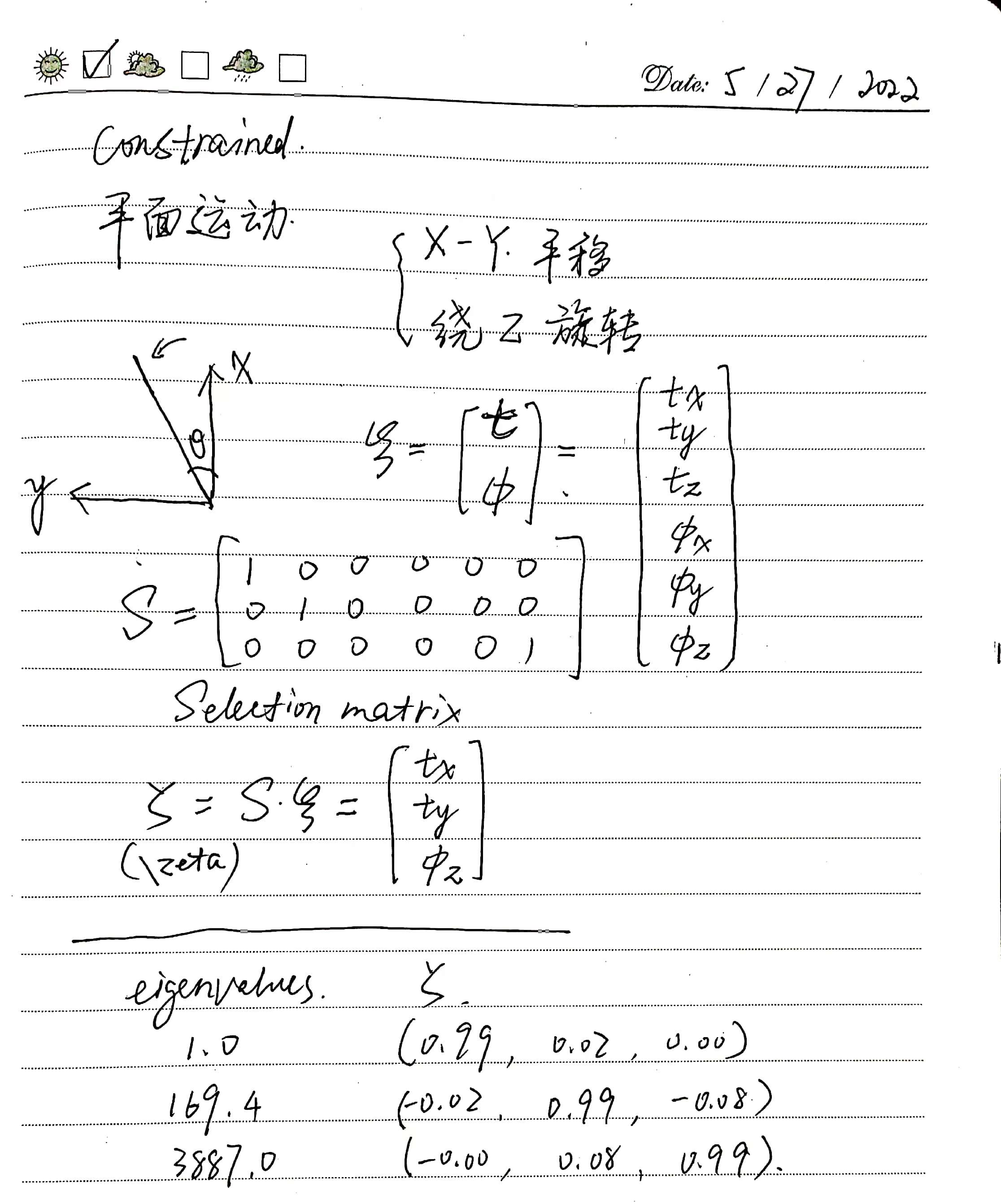
To test the extraction process of the two-dimensional pose subspace, use the following code.
// models/registration/registration_interface.cpp

bool RegistrationInterface::DetectDegeneration()
{
  Eigen::Matrix<float, 3, 6> selection = Eigen::Matrix<float, 3, 6>::Zero();
  selection(0, 0) = 1.0;
  selection(1, 1) = 1.0;
  selection(2, 5) = 1.0;

  for (std::size_t i = 0; i < hessian_eigenvectors_.cols(); i++) {
    Eigen::Vector3f zeta = selection * hessian_eigenvectors_.col(i);
		if(zeta.norm()<0.1) continue;
    std::cout << "\t" << std::fixed << hessian_eigenvalues_(i)
              << ",\t" << std::fixed << zeta.transpose() << std::endl;
  }
  std::cout << std::endl;

  return false;
}
The running results under non-degradation conditions are as follows.
#	eigenvalue,		\zeta (x,y,\theta)
	103.260437,	 	0.824976  0.561732 -0.061943
	151.702866,	 	0.564546 -0.823937  0.047920
	11549.036133,	-0.024072 -0.074255 -0.994592
The running results under degradation conditions are as follows:
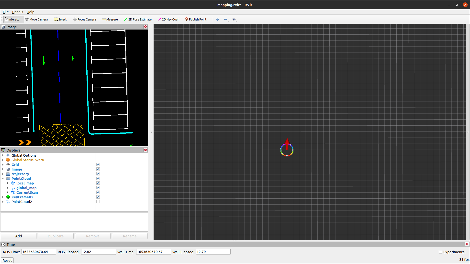
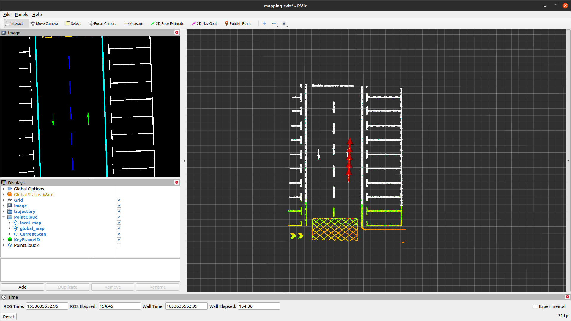
From the running results below, it can be observed that when only one lane line is detectable, localization degradation occurs in the direction of vehicle motion, specifically in the x-axis displacement direction.
#	eigenvalue,		\zeta (x,y,\theta)
	0.970717,	 	0.999650  0.026427 -0.000666
	186.364090,		-0.026334  0.994499 -0.088648
	4223.989258,	-0.001679  0.088677  0.995910
Discrepancy in Eigenvalues Corresponding to Translation and Rotation
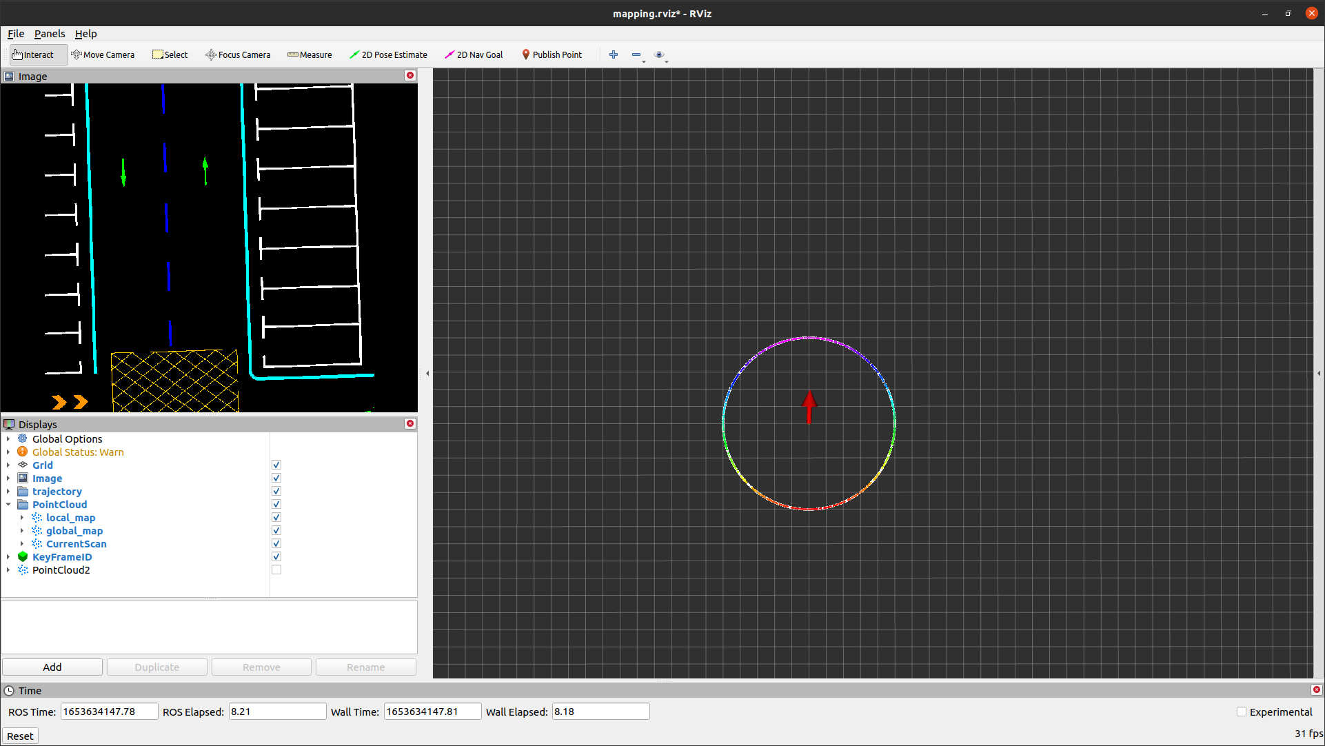
From the above results, it can be seen that there is a significant numerical difference in the eigenvalues corresponding to the translation and rotation directions in pose space. The fundamental reason for this issue lies in their inherent physical meanings and dimensions being different, which naturally results in numerical differences in the calculation of the Hessian matrix. To assess the impact of this difference on degradation determination, use the following code to generate point cloud data distributed in a circular pattern (to induce degradation in the rotational dimension) and observe and analyze the running results.
// data_pretreat/data_pretreat_flow.cpp
// bool DataPretreatFlow::LMRestructure()

  //for (int u = 0; u < img_height; u++) {
  //  for (int v = 0; v < img_width; v++) {
  //    rgb[0] = current_vision_data_.image[u * img_width * 3 + v * 3 + 2];
  //    rgb[1] = current_vision_data_.image[u * img_width * 3 + v * 3 + 1];
  //    rgb[2] = current_vision_data_.image[u * img_width * 3 + v * 3 + 0];
  //    std::map<unsigned long, unsigned char>::iterator it = semantic_label_map_.find(RGB2Key(rgb));
  //    if (it != semantic_label_map_.end()) {
  //      if (it->second != 5) continue;
  //      // semantic landmark pixels;
  //      current_cloud_data_.cloud_ptr->push_back(Pixel2Point(u, v, it->second, px_width, cx));
  //      mark[u][v] = 255;
  //    }
  //  }
  //}
	for(int i=0;i<1000;i++)
	{
		float radius=5.0;
		float angle=float(i)*M_PI*2.0/1000.0;
		float center_x=2.0, center_y=2.0;
		CloudData::POINTXYZI pt;
		pt.x=radius*cos(angle)+center_x;
		pt.y=radius*sin(angle)+center_y;
		pt.z=0.0;
		pt.intensity=1.999;
		current_cloud_data_.cloud_ptr->push_back(pt);
	}
Generate point clouds using five sets of parameters, and the running results are listed below respectively:
radius=1, center_x=0, center_y=0
#	eigenvalue,		\zeta (x,y,\theta)
	0.561985,		-0.000036 -0.000780 -1.000000
	219.874573,		-0.531902 -0.846806  0.000680
	234.954880,	 	0.846806 -0.531901  0.000385
radius=1, center_x=2, center_y=2
#	eigenvalue,		\zeta (x,y,\theta)
	0.061274,		-0.666107  0.667123 -0.333539
	218.766922,		-0.709544 -0.704620  0.007687
	2089.051025,	 0.229890 -0.241781 -0.942705

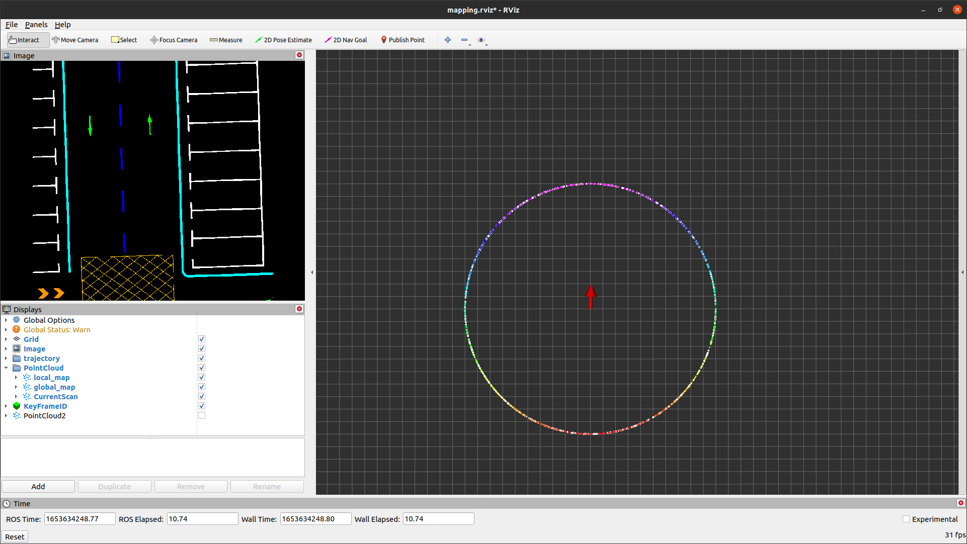
radius=5, center_x=0, center_y=0
#	eigenvalue,		\zeta (x,y,\theta)
	13.034241,		-0.000452 -0.000177  1.000000
	232.320877,		-0.419103 -0.907939 -0.000350
	248.135757,	 	0.907938 -0.419103  0.000336

radius=5, center_x=2, center_y=2
#	eigenvalue,		\zeta (x,y,\theta)
	1.442972,		-0.667143  0.666986 -0.331739
	234.465637,		-0.705799 -0.708396 -0.004888
	2236.154297,	 0.238263 -0.230880 -0.943359

radius=10, center_x=0, center_y=0
#	eigenvalue,		\zeta (x,y,\theta)
	52.092850,		-0.005853 -0.009619  0.999937
	229.914993,		-0.934878 -0.354857 -0.008886
	249.794281,		-0.354920  0.934871  0.006916

From the above results, it can be observed that even with point cloud data showing the same distribution, the numerical values of coordinates and the position of the vehicle center have a significant influence on the relative eigenvalues corresponding to the rotational and translational spaces. Although degradation conditions can be visually identified, such data differences pose significant challenges in developing quantitative evaluation procedures.
To address this issue, consider normalizing the coordinate values of point clouds when calculating the Hessian matrix, ensuring some level of comparability between rotational and translational spaces numerically.
The specific code modification is shown below. Lines 9-14 calculate the normalization scaling factor, and line 19 performs the normalization scaling of coordinate values.
// models/registration/registration_interface.cpp

RegistrationInterface::Matrix6f RegistrationInterface::GetCovariance()
{
  Eigen::Matrix3f R = cloud_pose_.linear();
  Eigen::Vector3f phi = Converter::Log(R);
  Eigen::Matrix3f J = ComputeJacobianSO3(phi);

  float ratio = 0.0;
  for (std::size_t i = 0; i < input_source_->size(); i++) {
    Eigen::Vector3f p(input_source_->at(i).x, input_source_->at(i).y, input_source_->at(i).z);
    ratio += p.norm();
  }
  ratio /= float(input_source_->size());

  Matrix6f hessian = Matrix6f::Zero();
  for (std::size_t i = 0; i < input_source_->size(); i++) {
    Eigen::Vector3f p(input_source_->at(i).x, input_source_->at(i).y, input_source_->at(i).z);
    Eigen::Matrix3f Rp_skew = Converter::toSkewSym(R * p / ratio);
    hessian.block<3, 3>(0, 0) += informations_[i];
    hessian.block<3, 3>(0, 3) += -informations_[i] * Rp_skew * J;
    hessian.block<3, 3>(3, 0) += J.transpose() * Rp_skew * informations_[i];
    hessian.block<3, 3>(3, 3) += -J.transpose() * Rp_skew * informations_[i] * Rp_skew * J;
  }
  hessian /= input_source_->size();

  Eigen::SelfAdjointEigenSolver<Matrix6f> es;
  es.compute(hessian);
  hessian_eigenvalues_ = es.eigenvalues().cwiseAbs();
  hessian_eigenvectors_ = es.eigenvectors();
  Matrix6f eigenvalues_inv = Matrix6f::Zero();
  for (int i = 0; i < 6; i++) {
    if (hessian_eigenvalues_(i) > 1e-7) {
      eigenvalues_inv(i, i) = 1.0 / hessian_eigenvalues_(i);
    }
  }
  Matrix6f hessian_inv = hessian_eigenvectors_ * eigenvalues_inv * hessian_eigenvectors_.transpose();

  Matrix6f cov = hessian_inv * GetFitnessScore();  // / float(input_source_->size());

  return cov;
}
After normalization, the running results are as follows.
From the results below, it can be seen that after normalization scaling, the eigenvalues show stronger comparability in numerical values.
radius=1, center_x=2, center_y=2
#	eigenvalue,		\zeta (x,y,\theta)
	0.032639,		-0.488264  0.487968 -0.723523
	216.304810,		-0.717490 -0.696418  0.014505
	459.038208,	 	0.496797 -0.526202 -0.690148

radius=5, center_x=0, center_y=0
#	eigenvalue,		\zeta (x,y,\theta)
	0.519825,		-0.000118 -0.000188 -1.000000
	236.314728,		-0.948404 -0.317065  0.000172
	244.470551,		-0.317065  0.948404 -0.000141
radius=5, center_x=2, center_y=2
#	eigenvalue,		\zeta (x,y,\theta)
	0.348308,	 	0.327198 -0.326727  0.886674
	234.227524,	 	0.778812  0.624642 -0.057223
	308.854462,		-0.535157  0.709276  0.458841

radius=10, center_x=0, center_y=0
#	eigenvalue,		\zeta (x,y,\theta)
	0.520339,		-0.000222 -0.000126 -1.000000
	230.980103,		-0.820820  0.571187  0.000110
	250.389847,		-0.571187 -0.820820  0.000230
#	eigenvalue,		\zeta (x,y,\theta)
	1.066867,		0.999544 0.030179 0.001228
	108.670120,	 	0.020603 -0.710965  0.702741
	286.107941,		-0.022054  0.701577  0.710928
#	eigenvalue,		\zeta (x,y,\theta)
	70.690025,	 	0.399140  0.641137 -0.655408
	133.363403,	 	0.909868 -0.351390  0.209567
	337.078064,		-0.095924 -0.681538 -0.724905
#	eigenvalue,		\zeta (x,y,\theta)
	2.656141,		0.685688 0.223352 0.692758
	134.606461,	 	0.283069 -0.958660  0.028918
	287.494446,		-0.670594 -0.176274  0.720573
Related Links
code: