MIT Challenge Dataset Pre-selection
Published:
MIT Challenge Dataset Pre-selection.
The MIT Challenge Dataset can be downloaded at Signal Enhancement for Magnetic Navigation Challenge Problem.
And this article is mainly quoted from the notebooks and reports of this repository.
Correlation Coefficients
The dataset has 92 different variables.
It is possible to find relationships between data using the Spearman correlation and the Pearson correlation.
- Pearson’s correlation aims to find linear relationships between data and
- Spearman’s correlation aims to find monotonic relationships.
Even though these are fairly simple relationships, it allows us to make an initial selection of variables with strong relationships between them.
Pearson correlation coefficient
\[\rho_{X,Y}=\frac{cov(X,Y)}{\sigma_X\sigma_Y}\]Pearson correlation coefficient is a measure of linear correlation between two sets of data. It is the ratio between the covariance of two variables and the product of their standard deviations. The value is between -1 and 1 where 1 represent a perfect correlation, -1 a perfect opposite correlation and 0 no correlation.
Spearman’s rank correlation coefficient
\[r_s=\rho_{R(X),R(Y)} =\frac{cov(R(X),R(Y))}{\sigma_{R(X)}\sigma_{R(Y)}}\]Spearman’s rank correlation coefficient is a nonparametric (distribution-free method) measure of [rank correlation](https://en.wikipedia.org/wiki/Rank_correlation) (ordering the labels of a specific variables). It assesses how well the relationship between two variables can be described using a monotonic function (a function that is entirely non-increasing or non-decreasing). The Spearman correlation between two variables is equal to the Pearson correlation between the rank values of those 2 variables. While Pearson correlation assesses linear relationship, Spearman’s correlation assesses monotonic relationships (wether linear or not). Same as Pearson correlation, the value is between -1 and 1 where 1 represent a perfect correlation, -1 a perfect opposite correlation and 0 no correlation.
\(\rho(\cdot)\) denotes the usual Pearson correlation coefficient, but applied to the rank variables.
Application
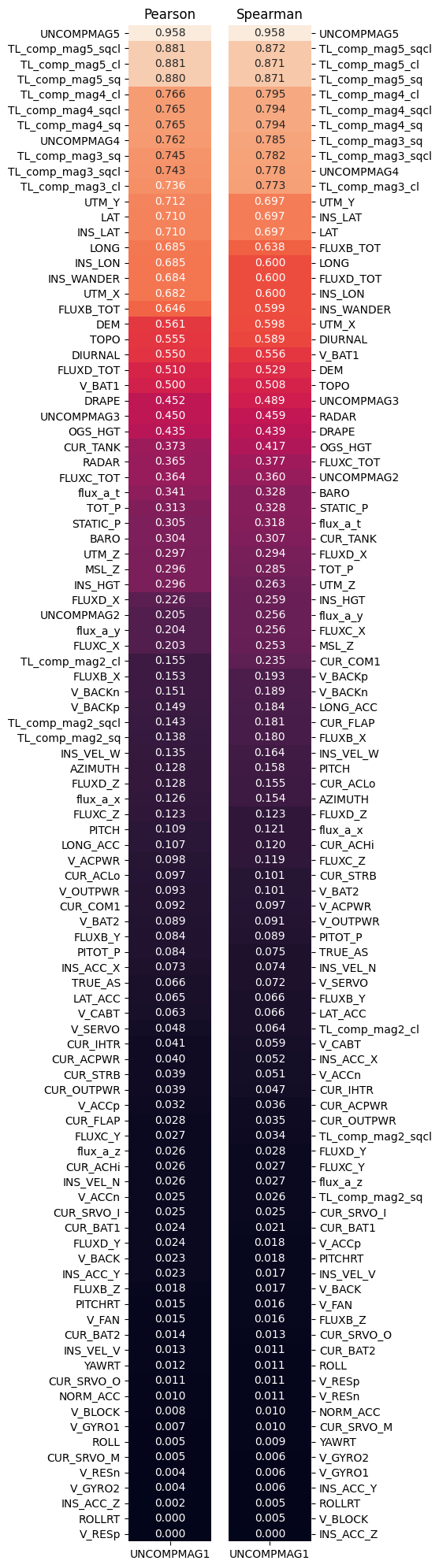
By applying these two correlations between the complete data set and magnetometer 1, which represents the ground truth, independently for each time sample:
on Flight 1003:
on Flight 1007:
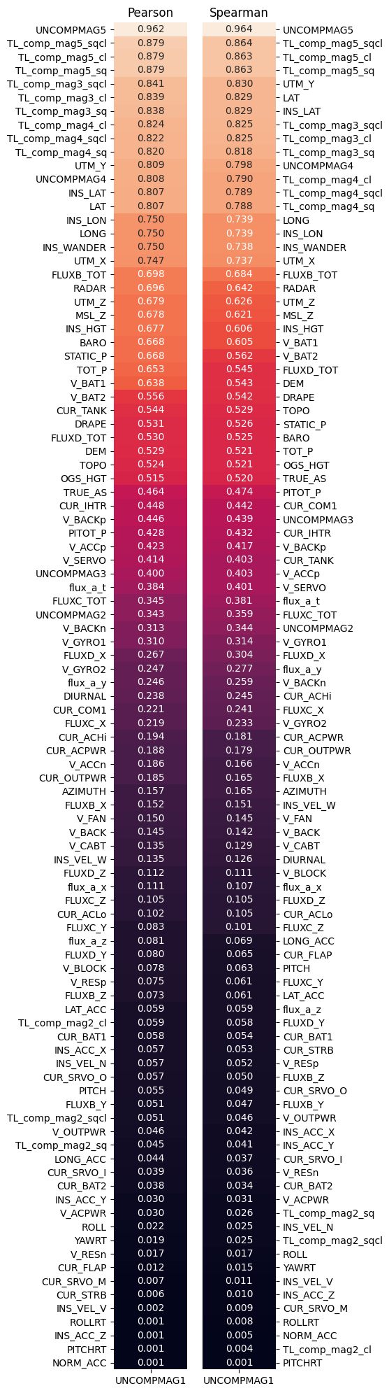
Before analyzing the results there are two points to consider :
- Pearson’s and Spearman’s correlations put forward linear or monotonic correlations. This means that there may be other more complex relationships between the variables that will not be highlighted here.
- The correlation above is between the truth (‘COMPMAG1’) and the other variables of the dataset. But the truth is based on a magnetometer at the end of a pole that aims to get as far away as possible from the effects of the plane. This means that the truth captures very little or no effect of the aircraft. To compensate for this, we take the magnetometers that are most correlated with the truth and then correlate the selected magnetometers with the other variables in the dataset.
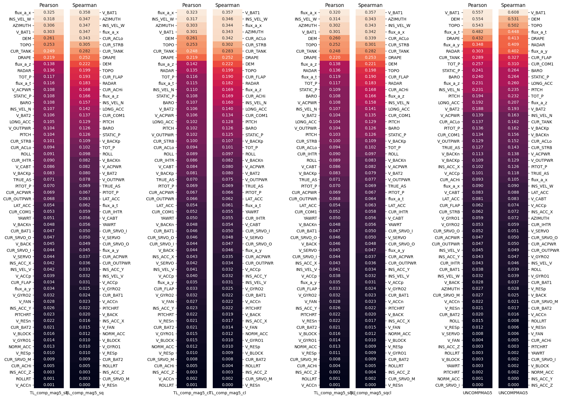
on Flight 1003:
on Flight 1007:
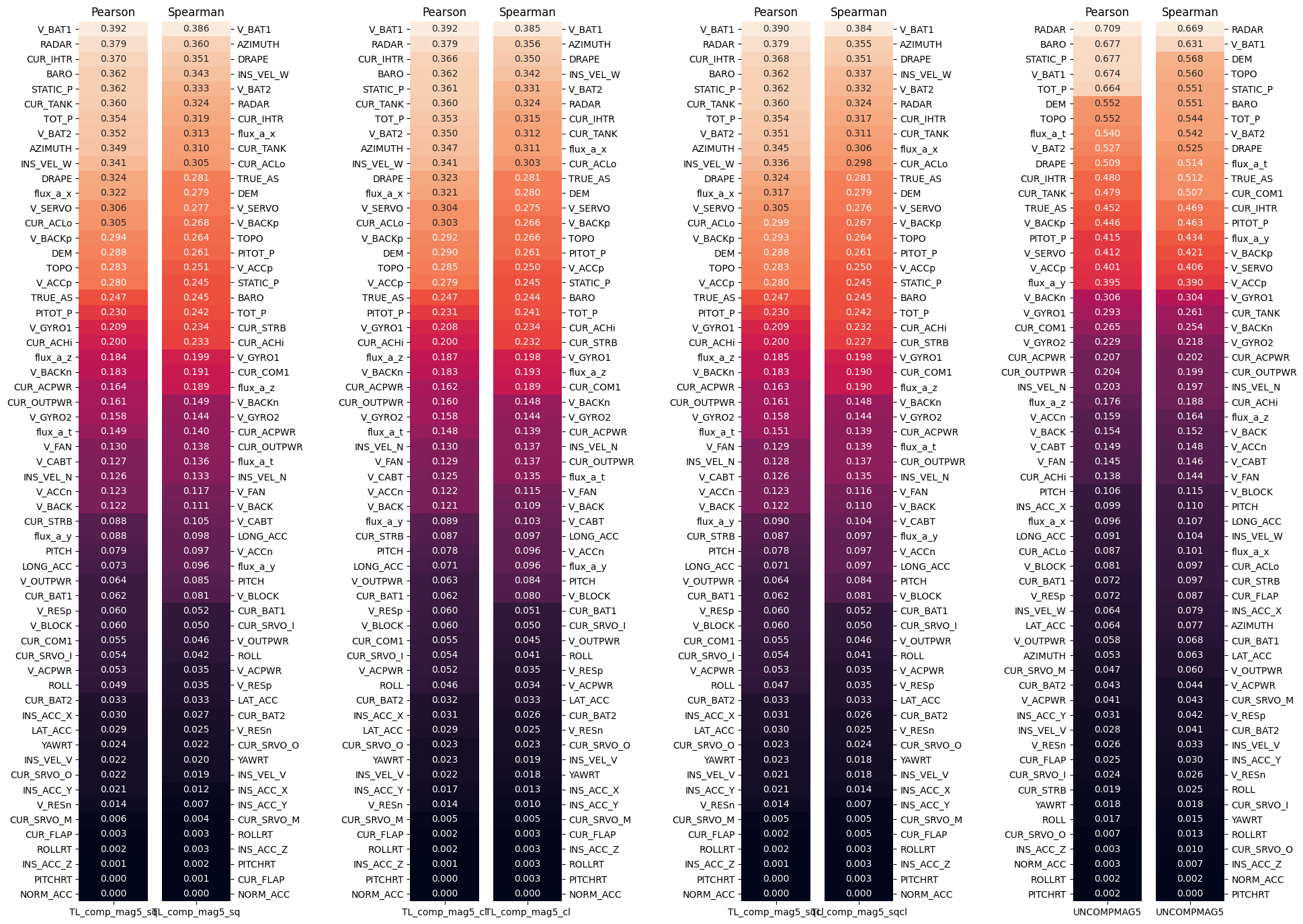
Several interesting facts stand out. First, the correlations between the variables and the Mag 5 are less strong with compensation than without, which seems logical because compensation reduces the effect of perturbations. The variable V_BAT1 is in the top 5 in each plot. This is very interesting because it means that battery 1 has an effect on the magnetometer measurements and therefore shows that the aircraft disturbs the measurements. The variables related to the INS also come up very often. The topography also seems to be an interesting element for the modeling. Let’s continue our analysis to see if the same variables emerge with other methods.
For both correlation methods, the variable V_BAT1 corresponding to the number one battery of the aircraft near the cockpit seems to have a strong correlation with the magnetometer 5. It is interesting to note that the variables related to altitude are correlated with the magnetometer (TOPO, DRAPE, RADAR, TOT_P), due to the fact that the increase in altitude acts as a low pass filter on our measurements
Mutual information
The mutual information (MI) of two random variables is a measure of the mutual dependence between the two variables. More specifically, it quantifies the "amount of information" obtained about one random variable by observing the other random variable. The concept of mutual information is intimately linked to that of entropy (average level of “information”, “surprise” or “uncertainty” inherent to the variable’s possible outcomes) of a random variable.
\[I(X;Y)=D_{KL}(P_{X,Y}\|P_X\otimes P_Y)\]Not limited to real-valued random variables and linear dependance like the correlation coefficient, MI is more general and determines how different the joint distribution of the pair (X, Y) is from the product of the marginal distributions of X and Y.
where
- \(D_{KL}\) is the Kullback-Leibler divergence \(D_{KL}(P\|Q)=\Sigma_{x\in\mathcal{X}}P(x)\log\left(\frac{P(x)}{Q(x)}\right)\)
- \(P_{X,Y}\) is the joint distribution of \(X\) and \(Y\);
- \(P_X\) and \(P_Y\) are the marginal distributions of \(X\) and \(Y\), respectively;
- \(\otimes\) is the tensor product.
When the MI is near 0, the quantities are independant. There is no upper bound but in practice values above 2 or so are uncommon (Mutual Information is a logarithmic quantity, so it increases very slowly).
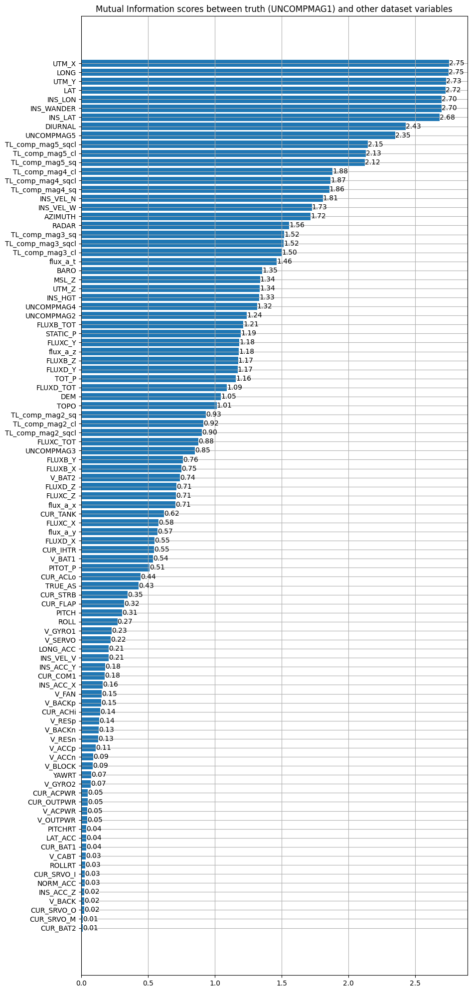
on Flight 1003:
on Flight 1007:
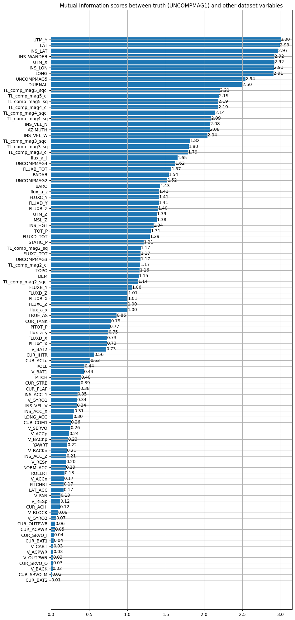
We look at the magnetometer most related to the truth then we choose it and look at the variables with which it has the most mutual information. We take again the magnetometer 5. We can also notice that the position (LAT,LONG) seems to share much information with the magnetic measurements. This is quite logical since each position in space is associated with a magnetic measurement.
Only a part of the data is displayed on this graph for readability reasons. The most interesting variables have a mutual information greater than 1. As before, magnetometer 5 is the most correlated magnetometer with the ground truth which is magnetometer 1. So, let’s reuse magnetometer 5 to compute the mutual information with the non-magnetic data of the dataset:
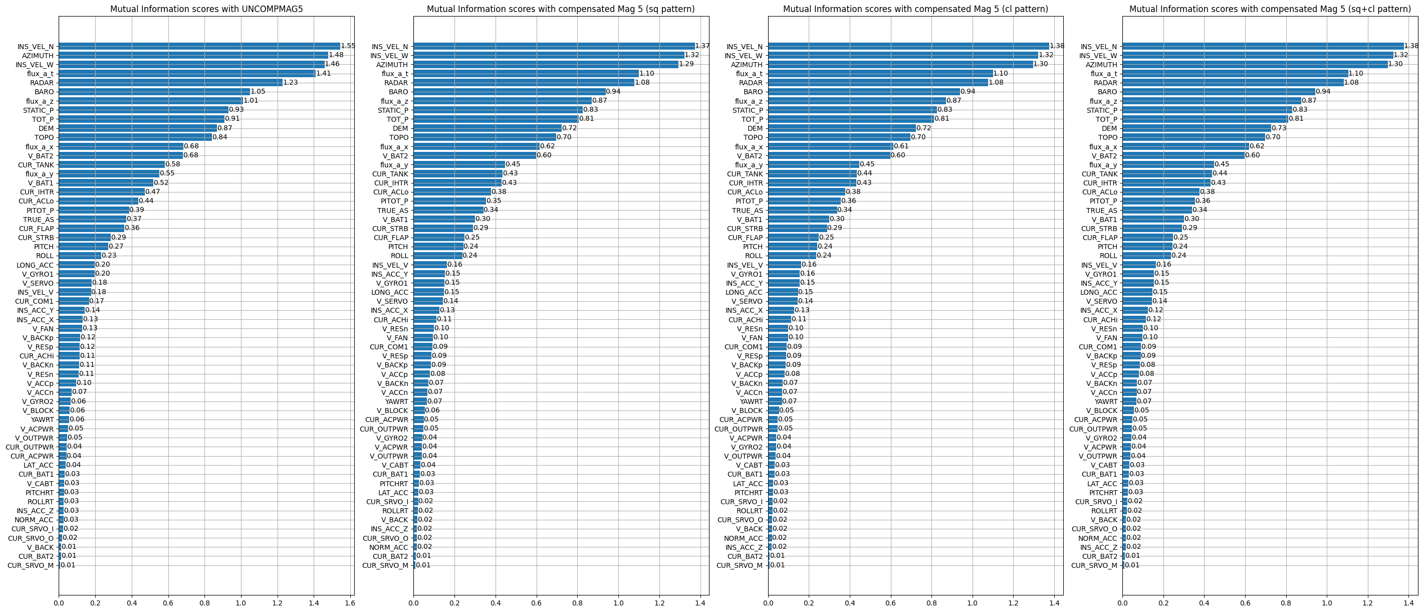
on Flight 1003:
on Flight 1007:
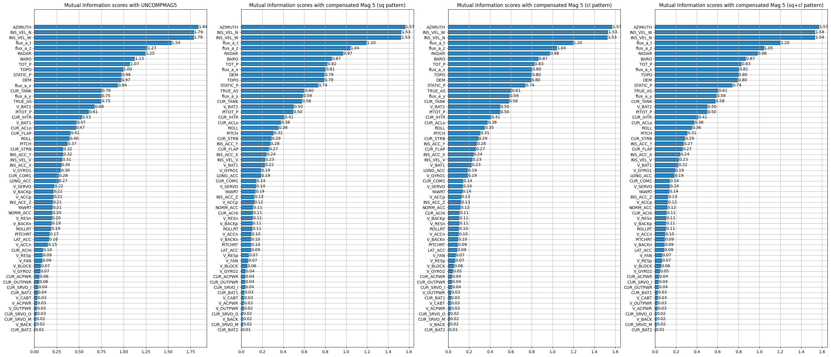
We can notice that some variables are similar to what we could obtain with the correlation like the velocities calculated by the INS or the variables related to the topography. We can also notice that pressure measurements brings information. As the altitude brings information on the measurements (the altitude has an impact on the intensity of the measurement), the pressure measurements also bring information because they are intimately linked to the altitude (the pressure decreases when the altitude increases and conversely). Some electrical measurements are also interesting like V_BAT which was already present in the correlation. In view of the previous results, it seems reasonable to think that large electrical elements close to the magnetometer have a direct impact on the measurements and that therefore the use of voltage/current measurements for a machine learning model will be useful to denoise the magnetometers. In comparison, the electrical effects created by the movements of the control surfaces do not seem to have much effect. This may be due to the fact that the magnetometer 5 is located relatively far from the control surfaces.
It can be seen from the graph that the aircraft orientation and speed variables appear to share information with the magnetic measurement from magnetometer 5. This is also the case for the altitude variables. **The "flux_a" variables are not considered because they correspond to the A vector magnetometer which is only available for flights 1006 and 1007.** This magnetometer cannot be considered as a training variable for our model. Some electrical variables also seem to have an impact, such as “CUR_TANK”. As a reminder, a description of all the variables in the dataset is available in Appendix B.
XGBoost
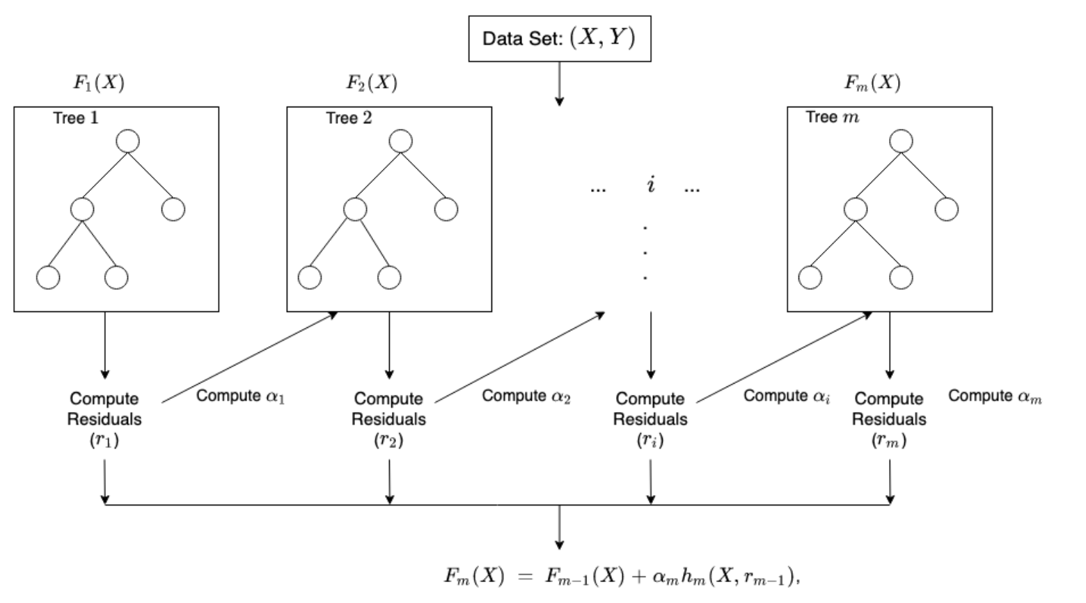
XGBoost (eXtreme Gradient Boosting) is an open-source software library which provides a regularizing gradient boosting framework. XGBoost provides a popular and efficient open-source implementation of the gradient boosted trees algorithm. Gradient boosting is a supervised learning algorithm, which attempts to accurtely predict a target variable by combining the estimates of a set of simpler, weaker models.
When using gradient boosting for regression, the weak learners are regression trees, and each regression tree maps an input data point to one of its leafs that containes a continous score. XGBoost minimizes a regularized (L1 and L2) objective function that combines a convex loss function (based on the difference between the predicted and target outputs) and a penalty term for model complexity (in other words, the regression tree functions). The training proceeds iteratively, adding new trees that predict the residuals or errors of prior trees that are then combined with previous trees to make the final prediction. It’s called gradient boosting because it uses a gradient descent algorithm to minimize the loss when adding new models.
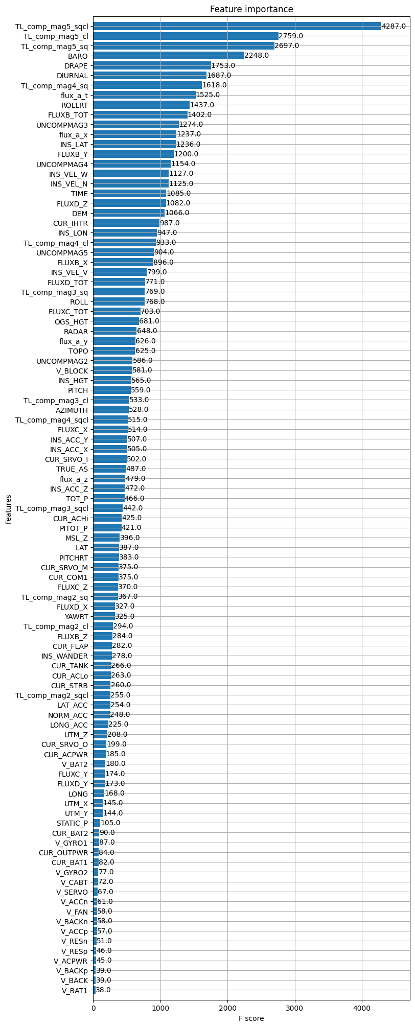
on Flight 1003:
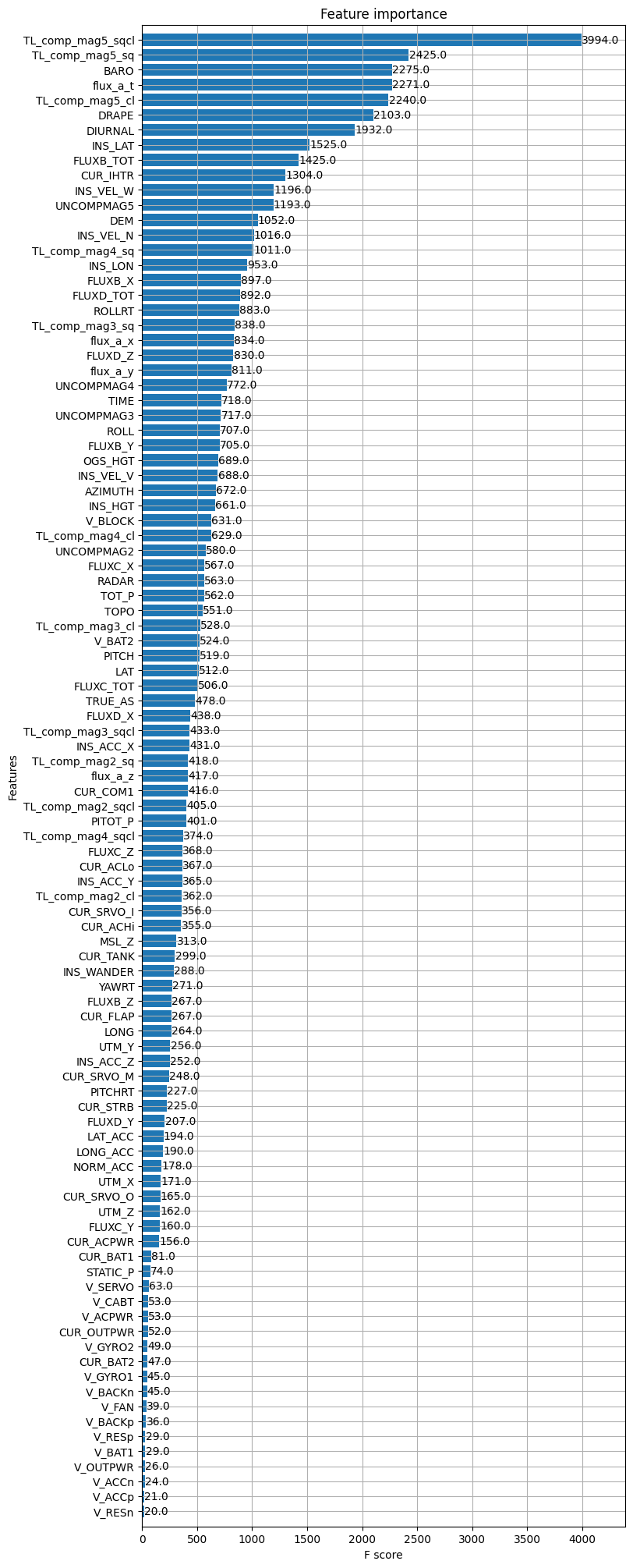
on Flight 1007:
First, if we look at the most important variables, we find the same as before with some exceptions. The measurement of the heater current of the INS seems to have a big impact also on the reconstruction of the truth. On the other hand, the impact of the batteries seems to be much less obvious than before.
We can see that XGBoost also allows to classify the importance of the magnetometers. The magnetometer 5 is of course first but more surprinsigly, it uses mainly the magnetometer 4 instead of the magnetometer 3. In correlation or mutual information, the border between the usefulness of magnetometer 3 and 4 is very thin but it is not the case here.
The model was trained to predict the magnetic anomaly (the variable IGRFMAG1) at time 𝑡 from the measurements in the dataset at time 𝑡. These measurements also include TL compensated magnetometers corrected by the IGRF model and diurnal effects. As with the previous methods, magnetometer 5 is the most useful variable for model prediction. Variables related to aircraft speed also stand out. An electrical variable also seems to have an impact, CUR_IHTR. The interesting variables are very close to those found with the previous methods.
Selected data for the models
After this data analysis, it is time to choose the features we will use for our model (they are not fixed and are subject to evolve). At first, the magnetometers 5 and 4 seem to be good choices for our model with a cloverleaf pattern. The magnetometer 2 is too noisy and the magnetometer 3 is noisier than magnetometer 4. As for the different features of the magnetometers, here is the list of what has been chosen:
V_BAT1/V_BAT2, CUR_IHTR, CUR_ACLo, CUR_TANK, CUR_FLAP These are all the selected electrical variables. These are the ones that seem most useful for debugging magnetometers.
INS_VEL_N/W/V Among all the analyses, the velocities calculated by the INS seem to correlate with our measurements. These features are therefore interesting for our model.
BARO The altitude is also an important element for our model. In the case of magnetic measurements, it acts as a low pass filter and therefore having the current altitude measurement is a relevant feature.
PITCH/ROLL/AZIMUTH Since to calibrate the effects of the aircraft we use the maneuvers of the control surfaces, it seems relevant to add the associated features. In the analyses, the link between the control surface movements and the magnetic measurements is not clear, but this mays be due to the fact that they are rather constant during the flight.
Training data
We now have our data for our training and we can start the model selection and the training of this model. However, our data are time series and, moreover, correspond to a spatial position. If we select all the lines of the flight 1003, we realize that some sections of the flight pass through the same places at different times. This leads to a potential leak of test data. Best example is flight 1003, section 1003.02 and 1003.04 correspond to the same trajectory at different times (but close enough in time to be considered identical).
In order to obtain relevant data for our models, we will choose flights 1002, 1003, 1004, 1006 and 1007. Flight 1005 is not taken into account because it may add too much data from magnetic measurement flights.
To validate the models correctly, two trainings will be realized :
- Training 1 : 1002, 1003, 1004, 1006 for train and 1007 for test
- Training 2 : 1002, 1004, 1006, 1007 for train and 1003 for test
This allows to validate the performance of the model on a flight it has never seen but also to validate it on several different flights.