MIT Challenge Dataset Description

MIT Challenge Dataset Description.

The MIT Challenge Dataset can be downloaded at Signal Enhancement for Magnetic Navigation Challenge Problem.

And this article is mainly quoted from A. R. Gnadt, “Advanced Aeromagnetic Compensation Models for Airborne Magnetic Anomaly Navigation,” Massachusetts Institute of Technology, 2022. , and also notebooks and reports of this repository.

MIT Challenge Dataset

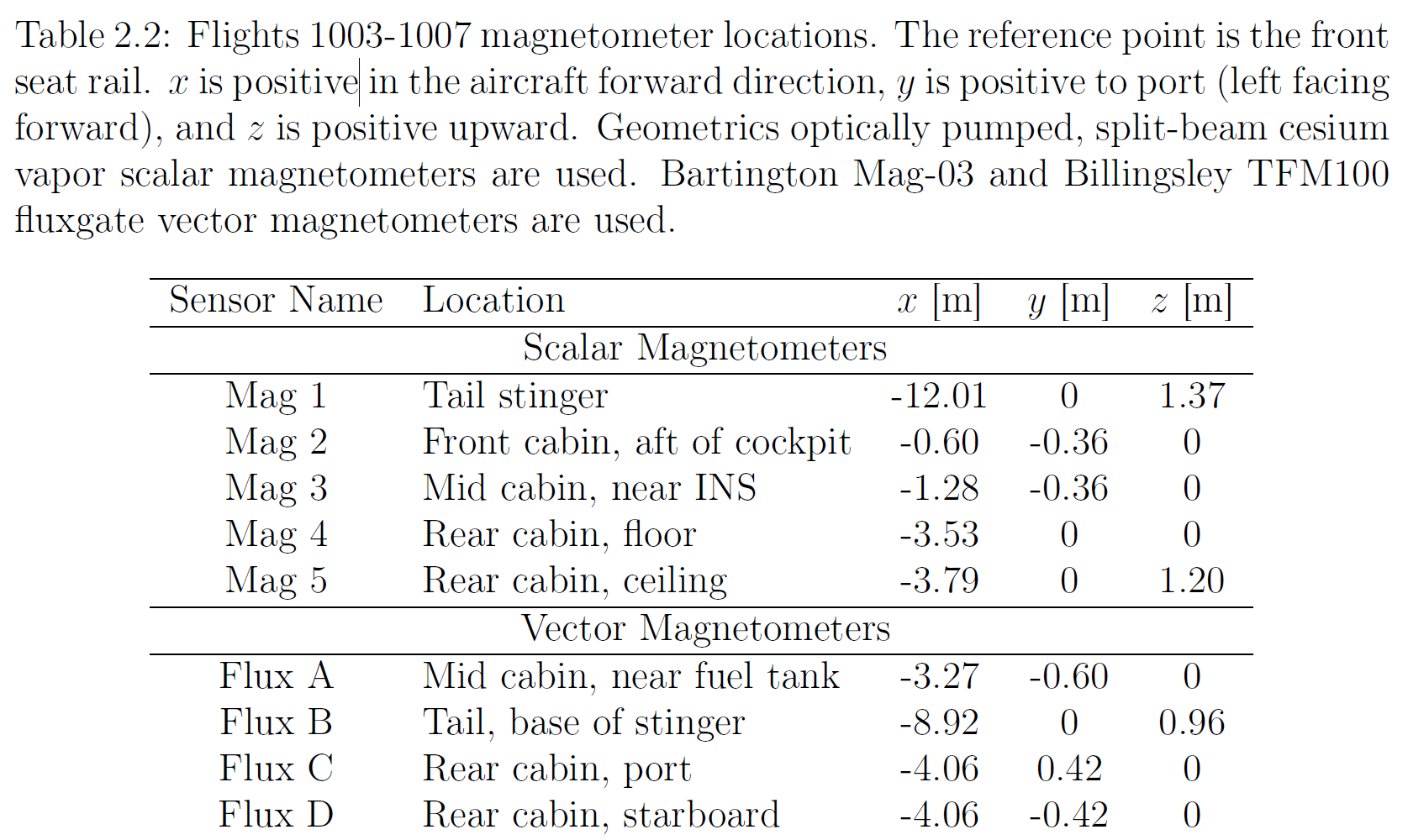
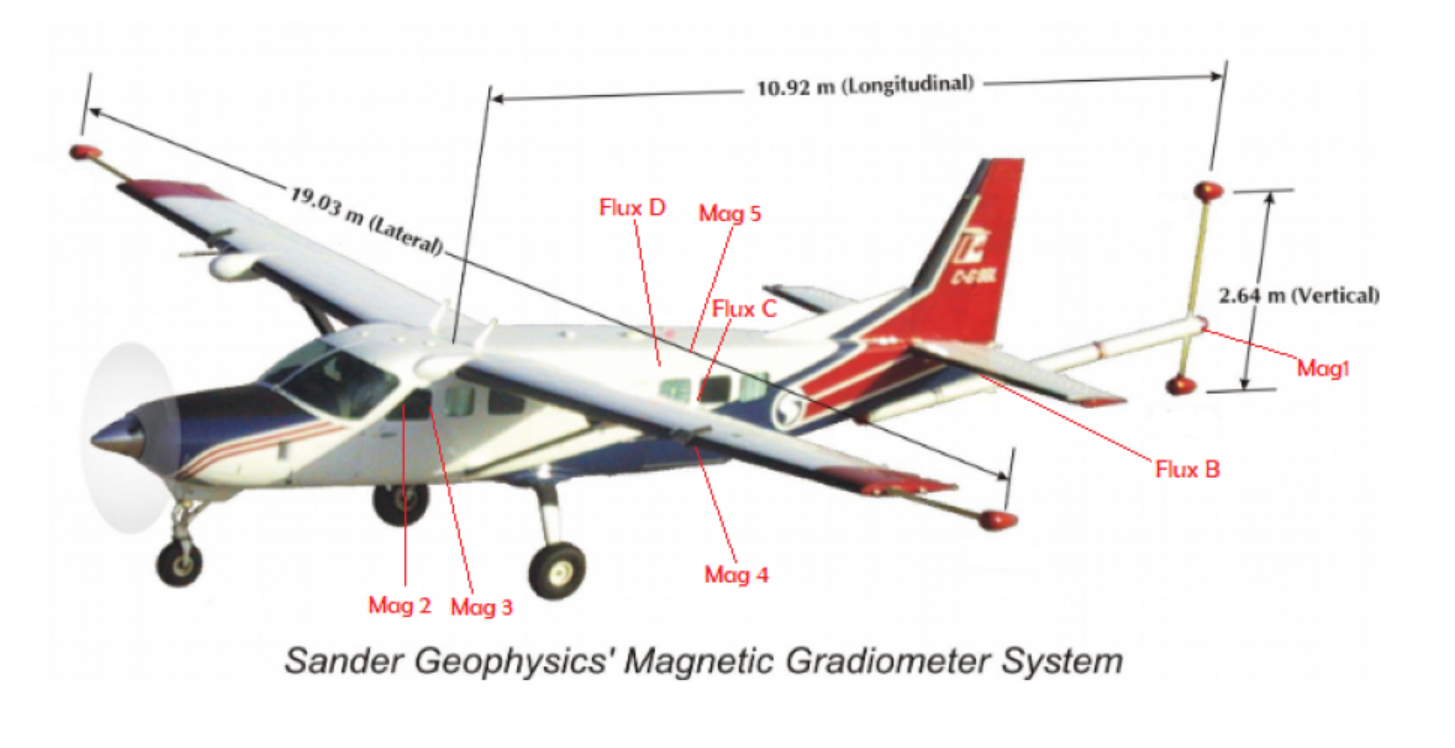
The Department of the Air Force Massachusetts Institute of Technology Artificial Intelligence Accelerator (DAF-MIT AI Accelerator) partnered with Sanders Geophysics Ltd. (SGL) to collect data over the Ottawa area in Ontario, Canada. They collected data from five scalar magnetometers placed at different locations on the aircraft, a Cessna 208B Grand Caravan, as well as from three vector magnetometers also placed at different locations on the aircraft. The scalar magnetic field data in the dataset used were measured using an optically pumped magnetometer. The vector magnetic field measurements were made using a Fluxgate magnetometer.

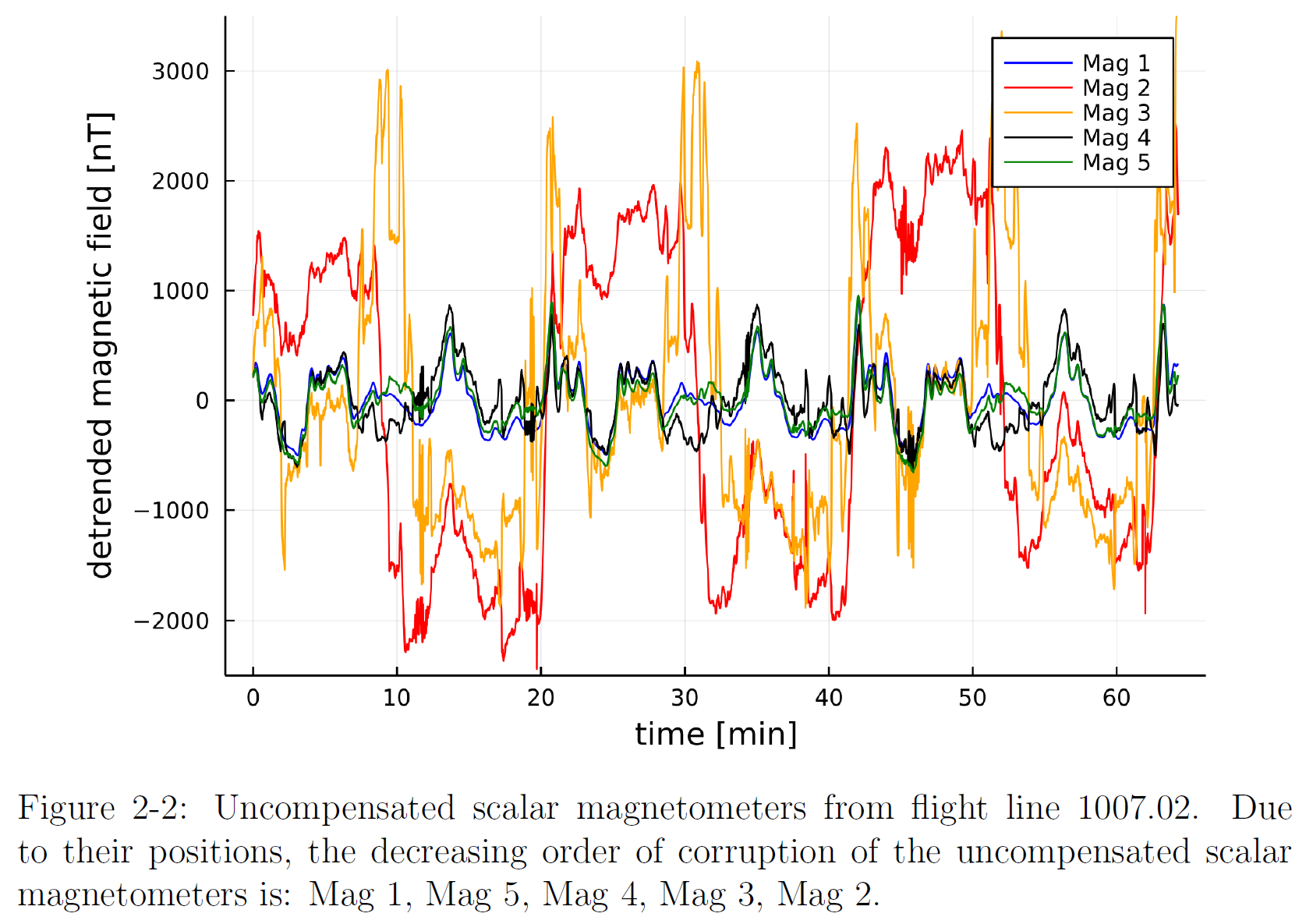
To provide a sense of the magnitude of corruption in the available scalar magnetometers listed in Table 2.2, an example of the uncompensated (raw) measurements is shown in Figure 2-2. Mag 1 has nearly no corruption, and Mag 5 follows the trend of Mag 1 well. Mag 4 is worse than Mag 5, but still largely matches the trend of Mag 1. Both Mags 2 and 3 have significant corruption and could not be used for MagNav without aeromagnetic compensation.

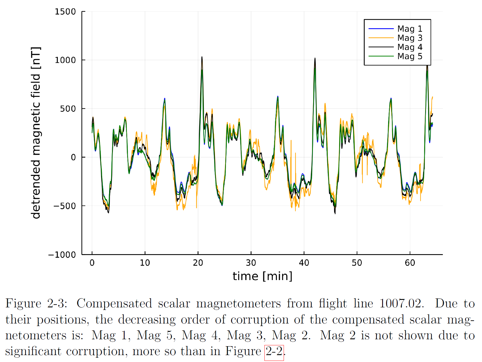
The scalar magnetometers can of course be compensated using a vector magnetometer, which is shown in Figure 2-3. Here, classical Tolles-Lawson aeromagnetic compensation (described in section 3.1) was performed on each scalar magnetometer using Flux A and the first calibration box of flight line 1006.04. Now Mags 3, 4, and 5 follow Mag 1 quite well, but decreasingly significant errors still remain for the respective magnetometers. Mag 2 performs worse after compensation, and is thus not shown for clarity.

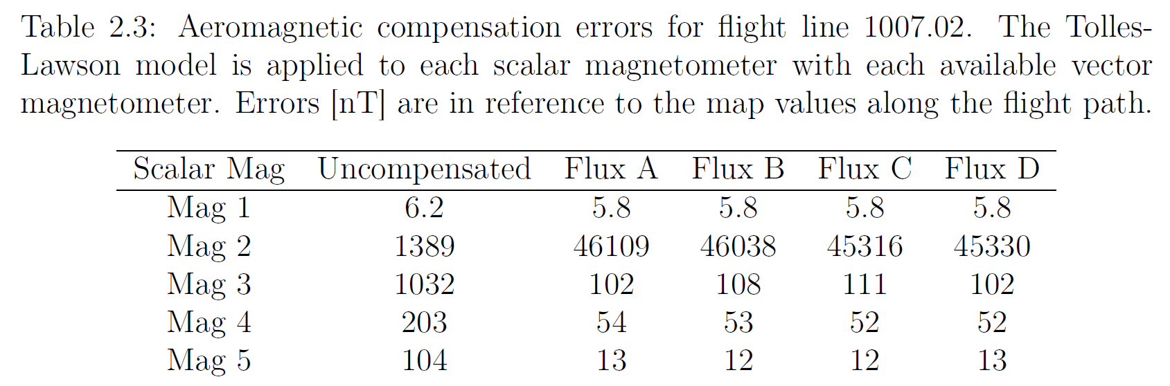
To emphasize the magnitude of corruption for each scalar magnetometer, the standard deviations of the magnetic errors are provided in Table 2.3. These errors are in reference to the magnetic anomaly map values along the flight path to give a sense of the errors that would be fed into the navigation algorithm. Comparing to the map values is not done in most of this work, since the tail stinger measurement is considered to be a better “truth” measurement as it was measured at the same time and avoids map errors. Mag 1 needs minimal compensation, while Mag 2 performs worse with compensation. The magnetic signal errors for Mags 3, 4, and 5 significantly decrease with compensation. Note that compensation performance is fairly insensitive to which vector magnetometer is used.

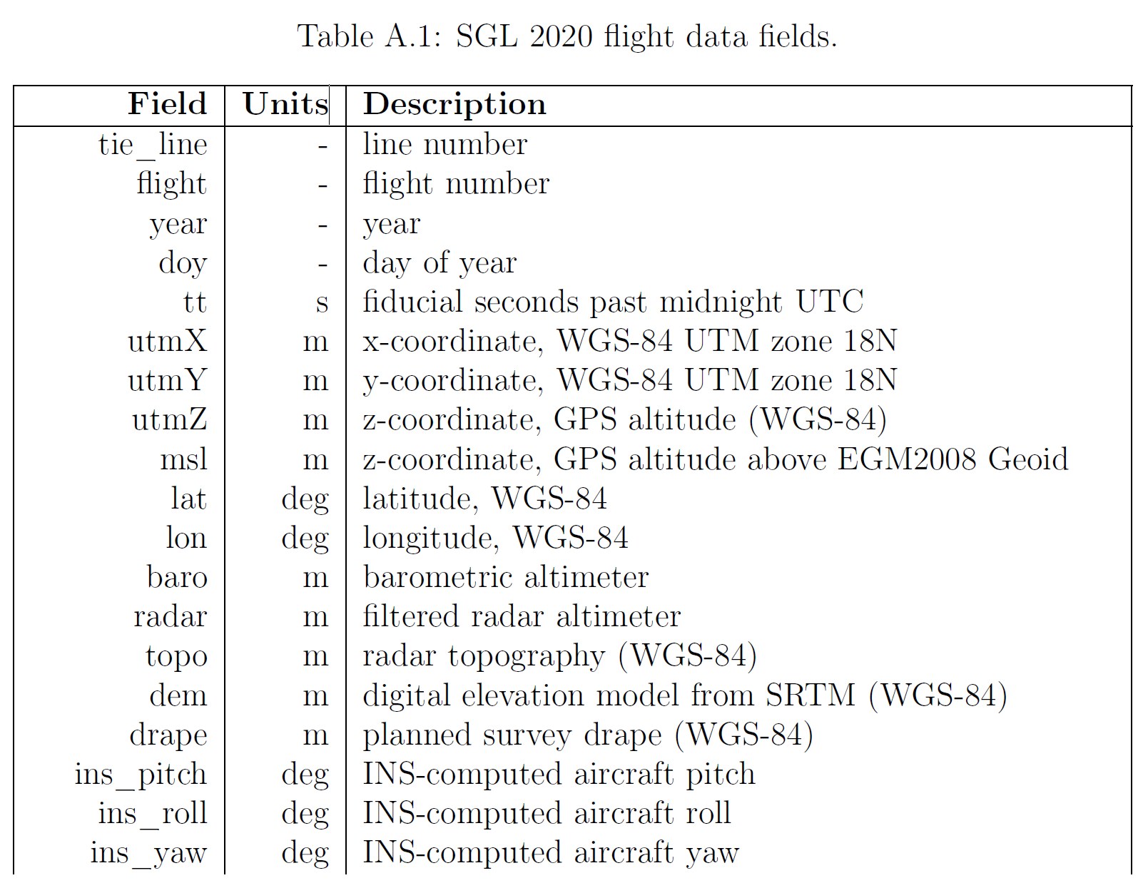
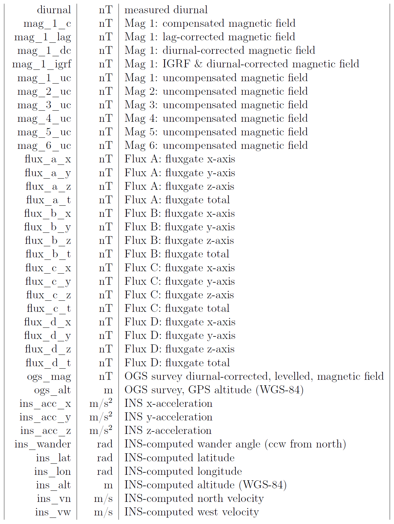
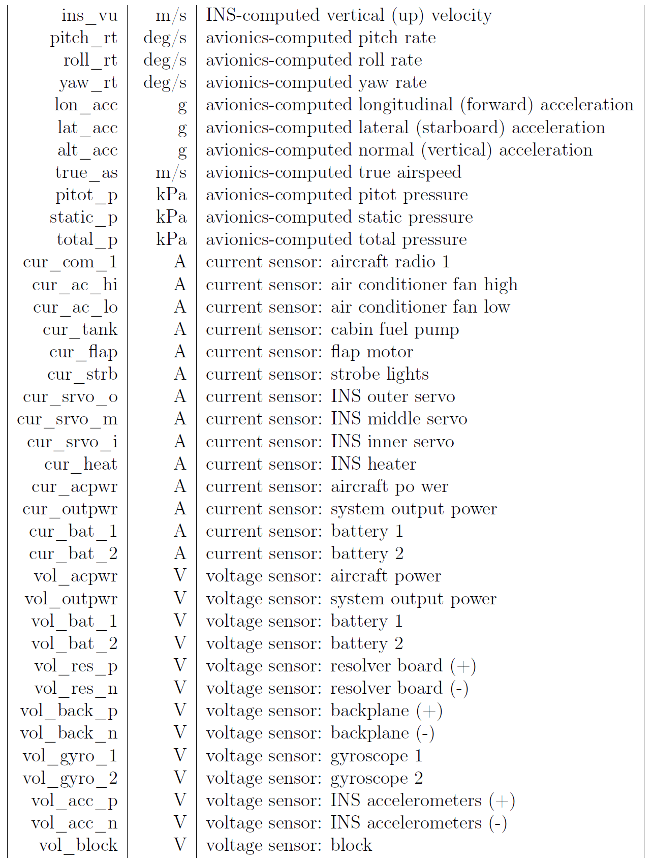
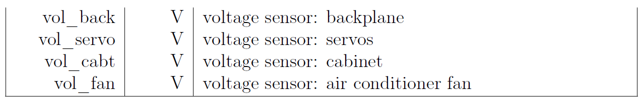
The flight data also contains supplemental sensor data from the inertial navigation system (INS), GPS position data, and auxiliary data from additional sensors, such as voltages and currents. This additional data reflects some of the temporal changes in the virtual magnetic dipole of the aircraft, which causes error in the magnetic data that is not removed with classical Tolles-Lawson compensation. Currents were measured using induction sensors (placed around wiring) rather than inline sensors due to additional approvals that would be required. This means the currents sensors may have picked up induced changes to wires’ electromagnetic fields that could have been caused by other sources. The full listing of the available data fields is shown in Appendix A. Note that when fitting or training any model, some data should not be used, especially **GPS position and tail stinger measurements**. In general the following data fields may be used: in-cabin magnetometer measurements and their gradients, diurnal and IGRF magnetic estimates, INS data, voltages, and currents.

During the data collection flights, various events were purposely carried out to cause temporal magnetic field disturbances during some flight lines. This included control surface movements (e.g. flaps up/down), fuel pump on/off, radio use, and movement of magnetic materials within the cabin. The flight patterns and altitudes were also varied from flight to flight to provide a diverse dataset. The flight altitudes were generally either at constant height above ellipsoid (HAE) or constant height above ground level (AGL), otherwise known as flying “on drape.” The former uses the altitude above an assumed perfect ellipsoid model of earth, while the latter uses the altitude on a drape surface above surface features, such as hills.

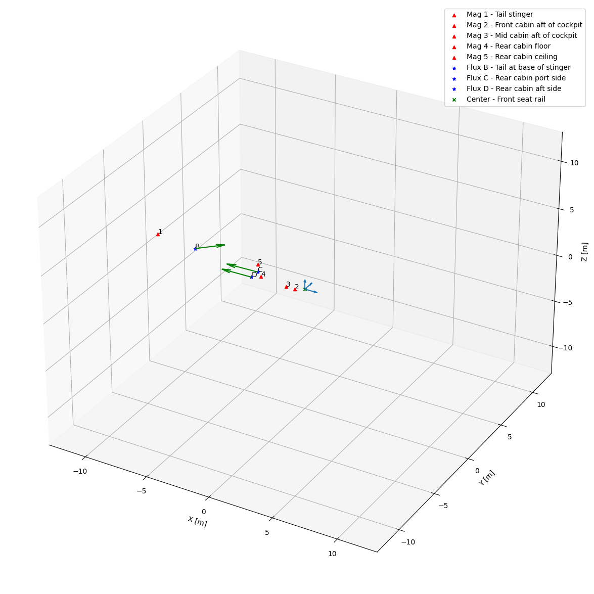
We have below a representation of their position in the plane as well as the possibility to vary the time to see the direction of the magnetic field measured by the vector magnetometers. The origin correspond to front seat rail.

time=47070.00

time=49000.00

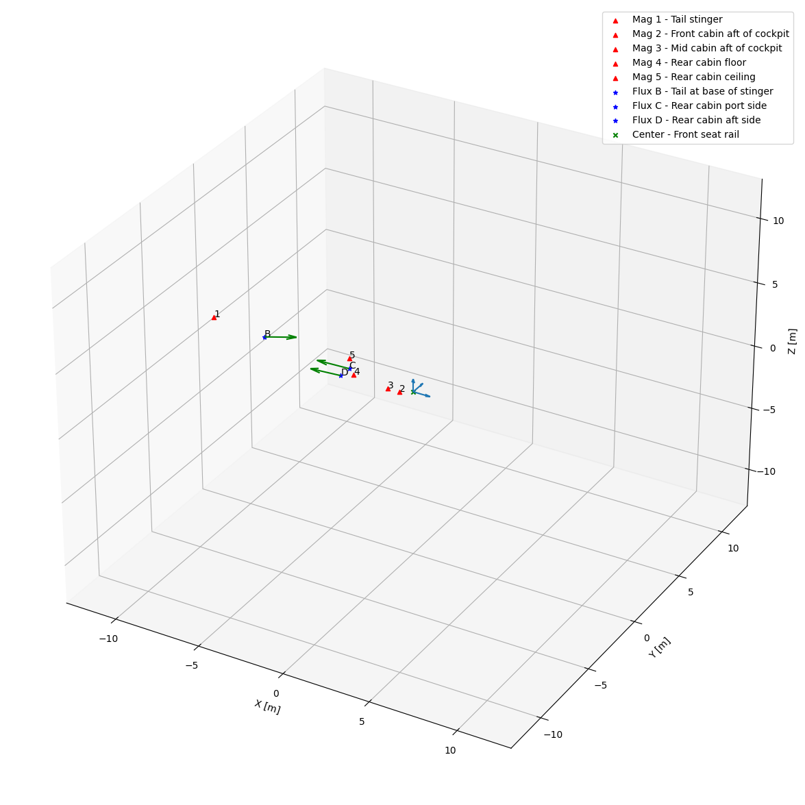
time=50000.00

Fitting/Training Flight Data

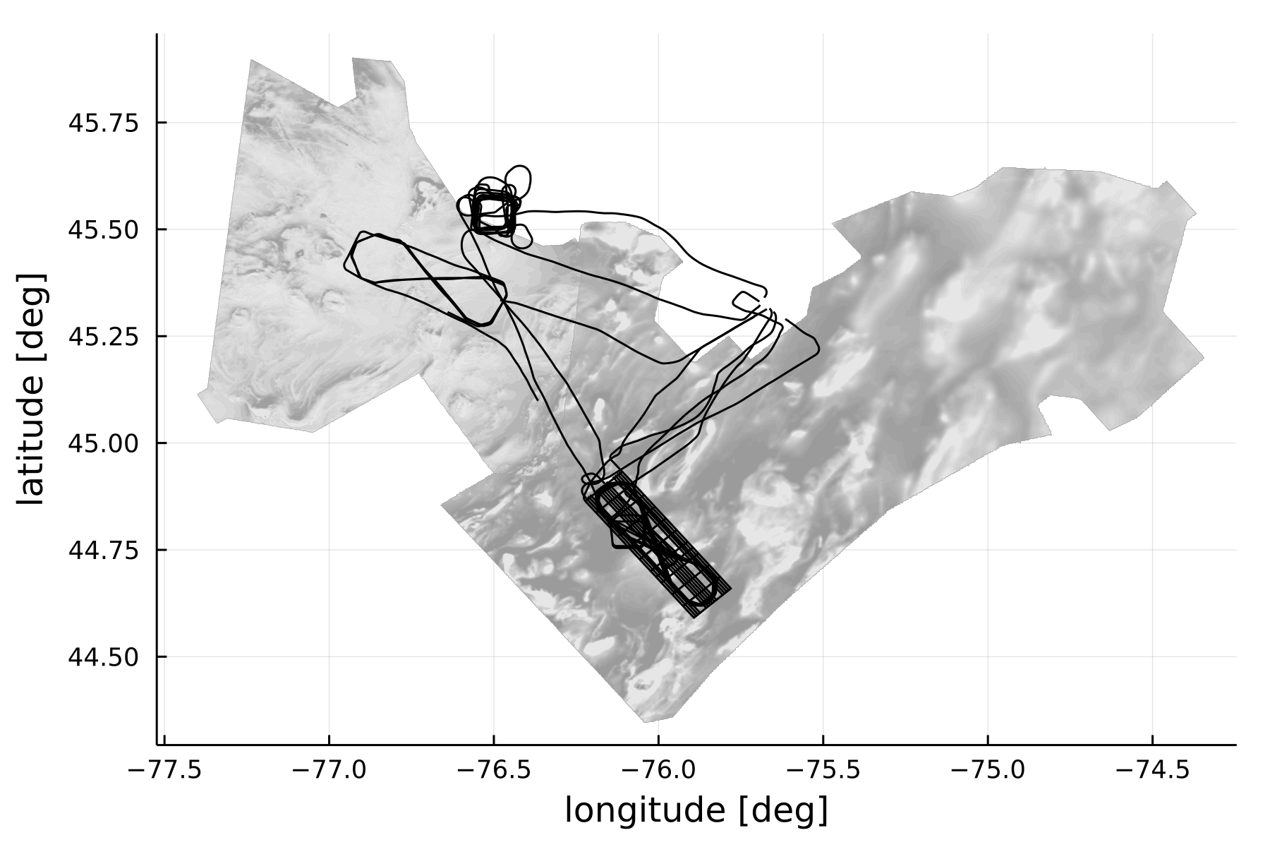
As previously mentioned, primarily data from flights 1003-1007 is used in this work. Up to approximately 11 hr and 52 min of this data was used for model training, which is shown in Figure 2-4.

Flight Descriptions

There are a total of 6 flights in the dataset.

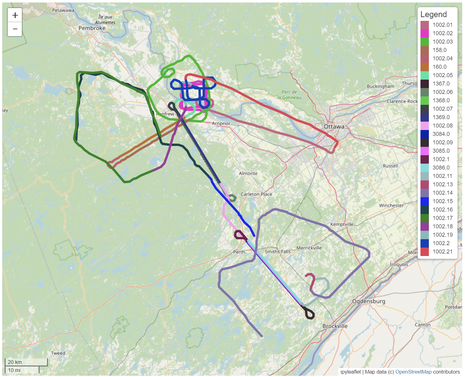
• Flight 1002 has two trim maneuvers and different flight paths to highlight the effects of the aircraft.
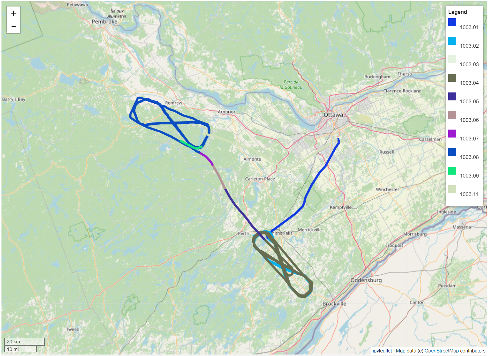
• Flight 1003 consists mainly of figure-of-eight trajectories.
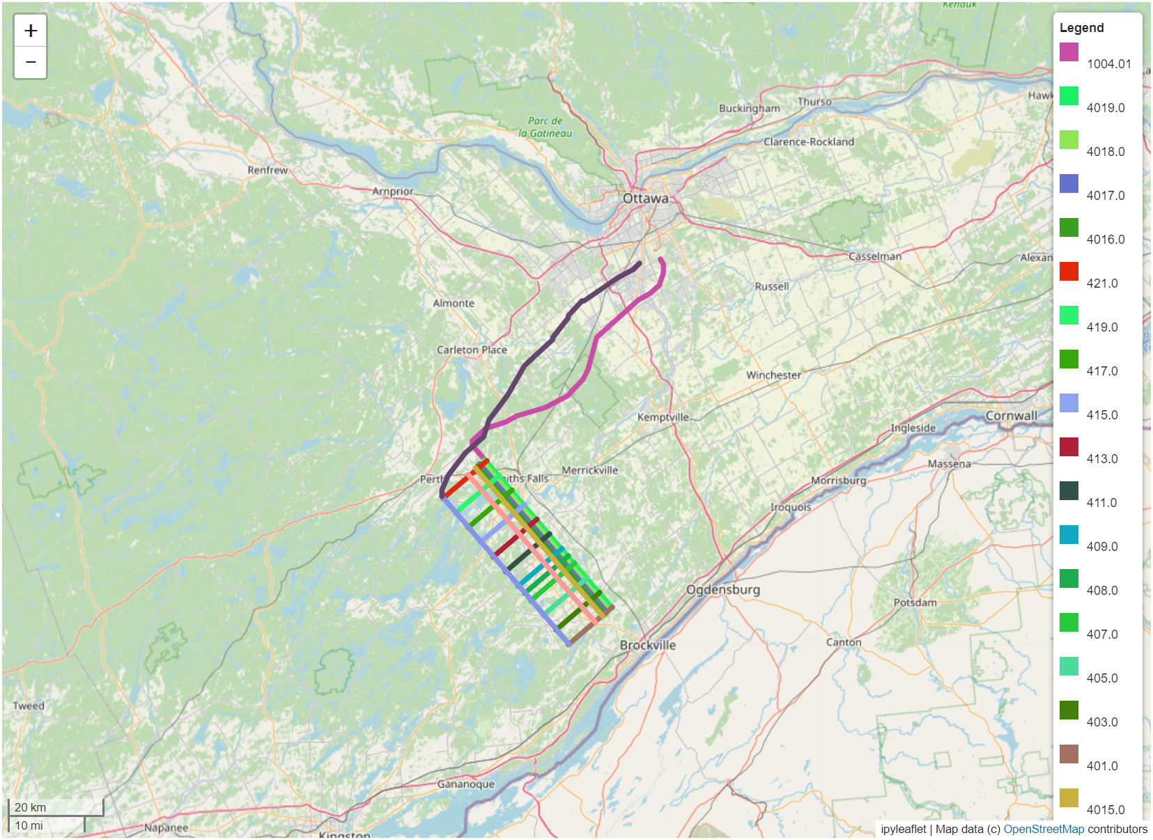
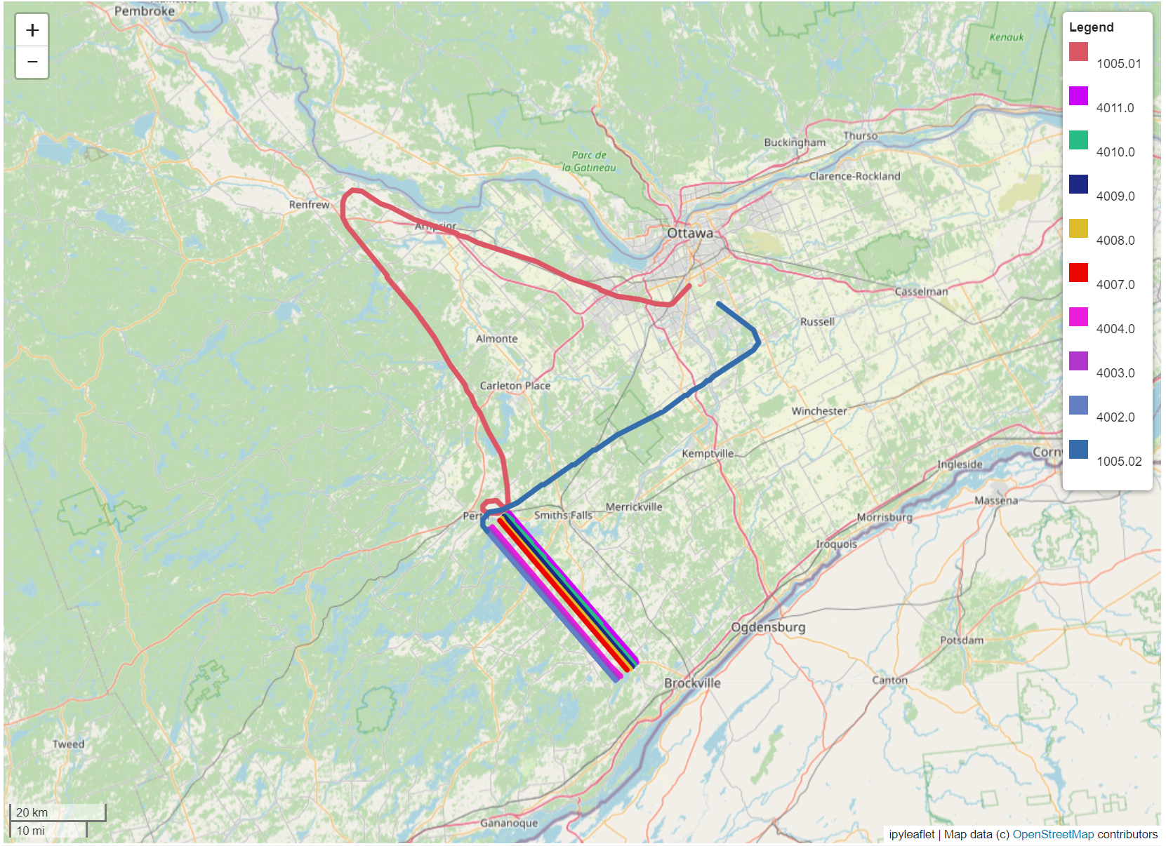
• Flights 1004 and 1005 are magnetic anomaly measurement trajectories for the purpose of creating anomaly maps.
• Flight 1006 has different compensation maneuvers and
• flight 1007 has different trajectories to highlight the different effects of the aircraft.

These different flights will serve as a basis for this work and are sufficiently representative of real trajectories to estimate the performance of the compensation methods used on real cases.

Flight : 1002 | Total flight time : 05h:45m:55s | Number of data collected : 207580 | Sampling frequency : 10.00Hz | Number of unique flight lines : 28
Flight : 1003 | Total flight time : 04h:26m:42s | Number of data collected : 160030 | Sampling frequency : 10.00Hz | Number of unique flight lines : 10
Flight : 1004 | Total flight time : 02h:15m:38s | Number of data collected : 81408 | Sampling frequency : 10.00Hz | Number of unique flight lines : 21
Flight : 1005 | Total flight time : 02h:16m:12s | Number of data collected : 81731 | Sampling frequency : 10.00Hz | Number of unique flight lines : 10
Flight : 1006 | Total flight time : 03h:00m:31s | Number of data collected : 108318 | Sampling frequency : 10.00Hz | Number of unique flight lines : 8
Flight : 1007 | Total flight time : 03h:10m:50s | Number of data collected : 114506 | Sampling frequency : 10.00Hz | Number of unique flight lines : 6

Flight 1002

Flight 1002 has two trim maneuvers and different flight paths to highlight the effects of the aircraft.

The objectives for Flight 1002 (see Flt1002_readme.txt) were to fly multiple calibration patterns and repeated survey lines, as well as free-fly within mapped regions. The flight began with a high altitude calibration maneuvers in the figure of merit (FOM) flight area over Shawville, Quebec. Then the aircraft flew 3 traverse lines and 2 control lines, in each of the Eastern Ontario and Renfrew flight areas, that had been flown in previous geomagnetic surveys. The purpose of this was to compare the repeat traverse and control lines to the original map data and look for measurement agreement. Additionally, this flight was used to determine that, since there was a trivial difference in accuracy between the traverse and control lines, the map is fully sampled. Starting near the south end of the Eastern Ontario traverse line, the aircraft completed a free-fly portion. This allowed for analysis regarding the amount that upward continuation of drape surface to constant altitude degrades the measurement quality. For this flight, the pilots purposely caused dierent magnetic events that were expected to alter the virtual dipole of the aircraft. Finally, the aircraft continued to free-fly while changing altitudes, conducted another set of calibration maneuvers, and completed the flight.

Flight 1003

Flight 1003 consists mainly of figure-of-eight trajectories.

Flights 1004 and 1005

Flights 1004 and 1005 are magnetic anomaly measurement trajectories for the purpose of creating anomaly maps.

The objective for Flights 1004 and 1005 (see Flt1004_readme.txt and Flt1005_readme.txt) was to create a small, high resolution, recently-flown magnetic anomaly map (the Perth mini-survey) for future comparison and navigation work. A small survey was flown in the Eastern Ontario flight area at 800m. The line spacing was less than the height above ground level (AGL) to ensure that the generated map is fully sampled.

Flights 1004 and 1005 are in fact magnetic map measurement flights, which explains the long lines close together.

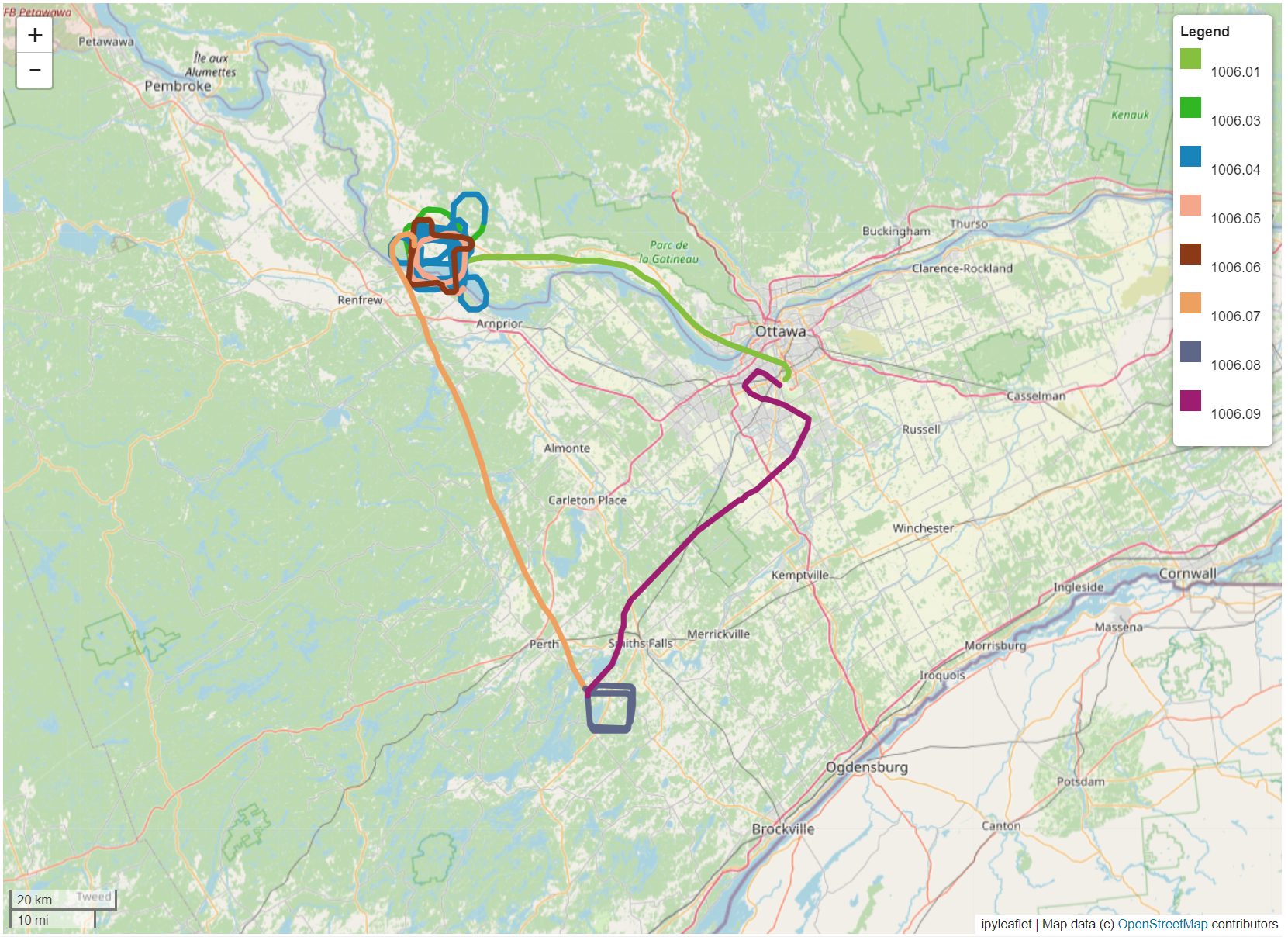
Flight 1006

Flight 1006 has different compensation maneuvers.

The objective for Flight 1006 (see Flt1006_readme.txt) was to fly a variety of calibration maneuvers at various altitudes. This included calibration patterns in the FOM flight area at progressively higher altitudes, as well as a low altitude calibration pattern in the Eastern Ontario flight area at 400m. Throughout the flight, the magnetic state of the aircraft was varied.

Flight 1006 represents several trim maneuvers made at different altitudes and with different shapes. It is also interesting to note that some sections of the trajectories are cut off. These sections have been removed by the creators of the dataset either due to erroneous measurements or in order to keep these sections as test data for the challenge.

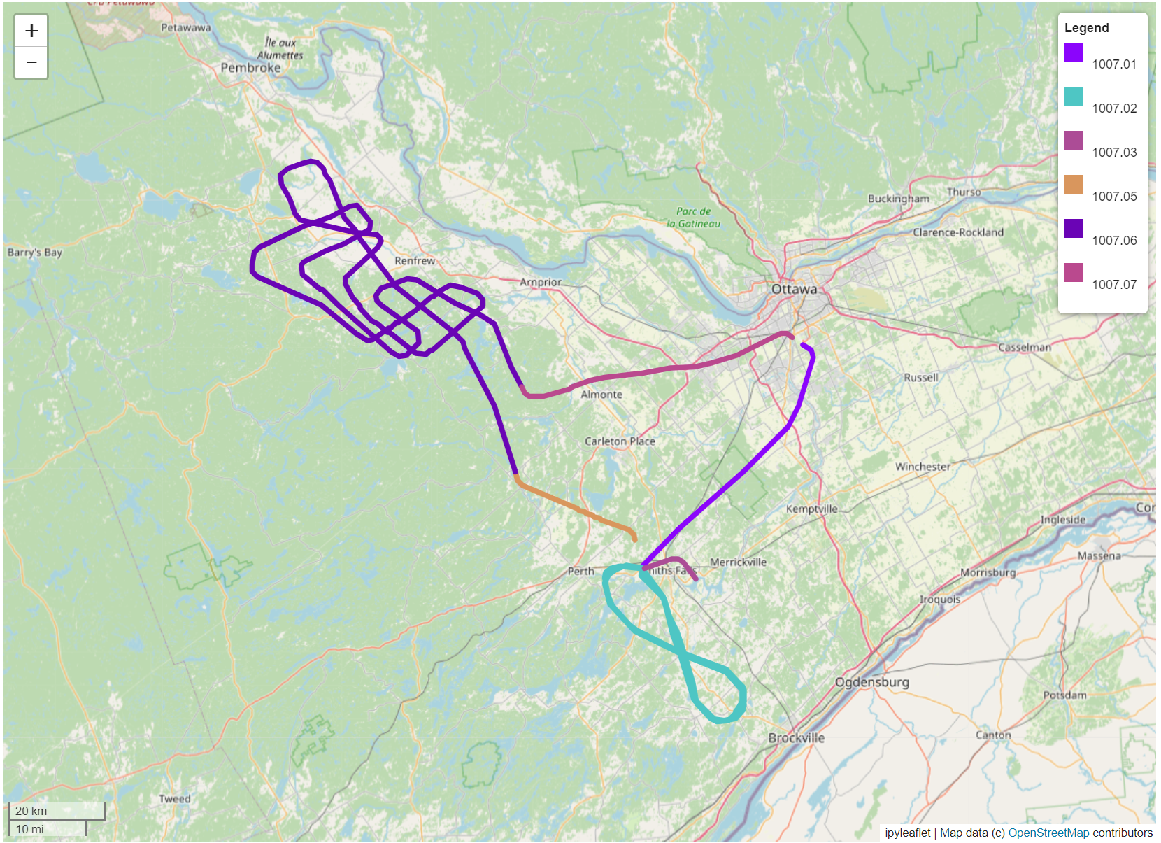
Flight 1007

flight 1007 has different trajectories to highlight the different effects of the aircraft.

The objective for Flight 1007 (see Flt1007_readme.txt) was to free-fly in the Perth mini-survey at 800m and the Eastern Ontario and Renfrew flight areas at 400m.

The most interesting flight seems to be flight 1007. It has different and slightly more complex trajectories than a simple straight line. Section 1007.04 serves as a test section for the challenge, which is why this section is not available.

SGL Flight Data Fields