Tolles-Lawson Model-based Aeromagnetic Compensation
Date:
Background
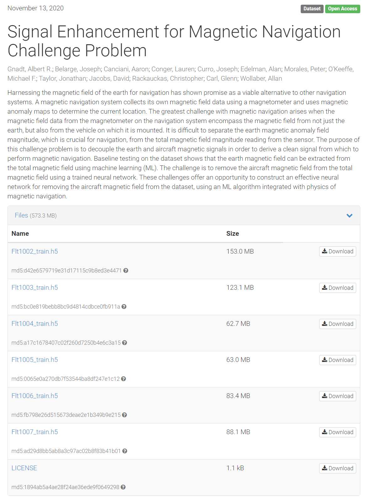
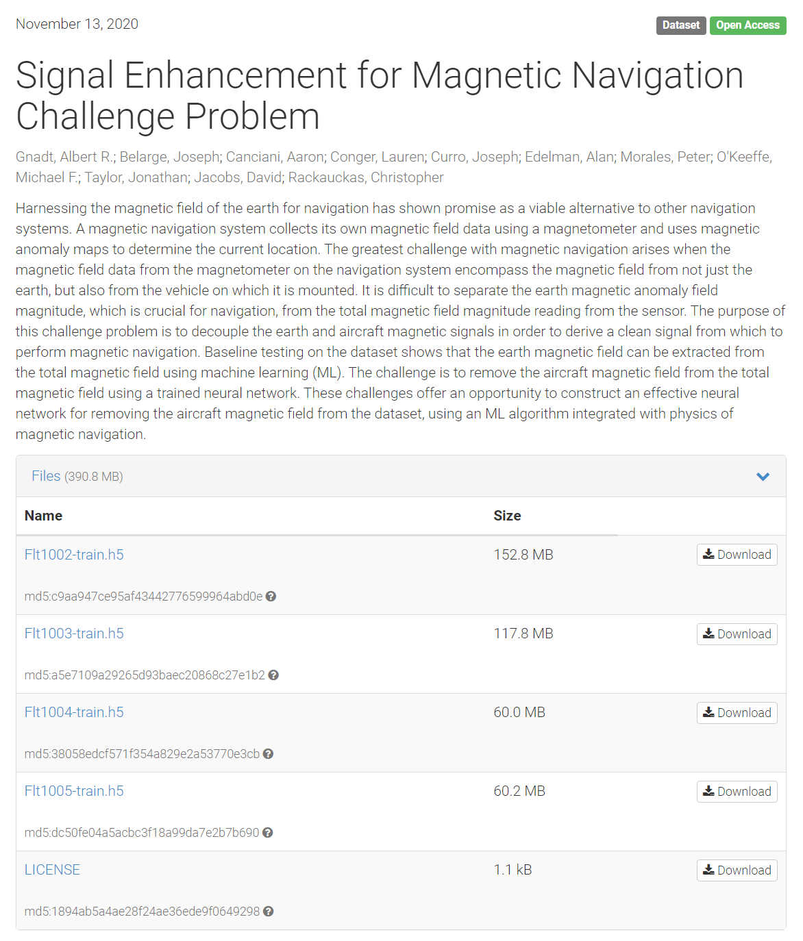
For more details, please refer to the Signal Enhancement for Magnetic Navigation Challenge Problem.
The best submission to date was submitted by: Ling-Wei Kong, Cheng-Zhen Wang, and Ying-Cheng Lai from Arizona State University (submission).
Dataset Version Issue
There are two versions of the dataset: Version 1 and Version 2.
Both versions contain the same collected data, but they differ in file organization, including data naming and storage order.
Caution should be exercised when using them.
Tolles-Lawson Model-based Aeromagnetic Compensation
The measured magnetic field inside the cabin consists of two components, which can be represented as
\[\vec{B}_t=\vec{B}_e+\vec{B}_a\]Where:
- \(\vec{B}_t\) represents the measured magnetic field vector inside the cabin.
- \(\vec{B}_e\) represents the Earth’s magnetic field, including the main field, anomaly field, and diurnal field.
- \(\vec{B}_a\) denotes the unknown carrier-induced magnetic interference field.
According to the Tolles-Lawson model assumptions, the carrier-induced magnetic interference field is composed of the permanent magnetic field, induced magnetic field, and eddy current magnetic field, namely
\[\vec{B}_a=\vec{B}_{perm}+\vec{B}_{ind}+\vec{B}_{eddy}\]Permanent magnetic fields can be modeled as
\[\vec{B}_{perm}=\boldsymbol{a}= \begin{bmatrix} a_1 \\ a_2\\ a_3 \end{bmatrix}\]The permanent magnetic moment terms represent nearly constant permanent magnetization of various ferromagnetic components, including both the carrier itself and items within the carrier. These terms do not change unless there is a change in the carrier’s configuration or contents.
The induced magnetic moment terms can be expressed as
\[\vec{B}_{ind}=\boldsymbol{b}\vec{B}_t= |\vec{B}_t| \begin{bmatrix} b_{11} & b_{12} & b_{13} \\ b_{21} & b_{22} & b_{23} \\ b_{31} & b_{32} & b_{33} \end{bmatrix} \hat{B}_t\]The induced terms involve six unknown coefficients. The induced magnetic moment terms represent the secondary magnetic field induced by the Earth’s field in magnetic susceptible components of the carrier. The magnitude and direction of induced magnetization depend on the relative orientation between the carrier and the Earth’s field. Since the aircraft structure is primarily composed of non-magnetic aluminum alloys, the main source of induced magnetic field is the aircraft engines.
Note: There is an approximation here, where the observable quantity \(\vec{B}_t\) is used instead of the unknown \(\vec{B}_e\). For details, see here.
The eddy current magnetic moment terms can be expressed as
\[\vec{B}_{eddy}=\boldsymbol{c}\dot{\vec{B}}_t= |\vec{B}_t| \begin{bmatrix} c_{11} & c_{12} & c_{13} \\ c_{21} & c_{22} & c_{23} \\ c_{31} & c_{32} & c_{33} \end{bmatrix} \dot{\hat{B}}_t\]The eddy current terms involve nine unknown coefficients. Eddy currents represent circulating currents induced by the time-varying Earth’s field (relative to the carrier) interacting with conductive components of the carrier. Unlike fixed and induced magnetic fields, the eddy current magnetic field depends on the rate of change of magnetic flux through these components over time, such as the carrier’s outer shell. The magnetic field generated by eddy currents follows Faraday’s law, opposing the fields that produce them, similar to the principle of inducing current in a coil rotating in a uniform magnetic field.
Based on the parameterization above, the interference magnetic field can be represented as
\[\vec{B}_a=\boldsymbol{a}+\boldsymbol{b}|\vec{B}_t|\hat{B}_t+\boldsymbol{c}|\vec{B}_t|\dot{\hat{B}}_t\]Here, the parameters \(\boldsymbol{a,b,c}\) together contain 21 coefficients in total, but due to the symmetry of the induced magnetic moment matrix, in the standard Tolles-Lawson model, there are a total of 18 unknown coefficients.
\[\vec{B}_a= \begin{bmatrix} \beta_1 \\ \beta_2\\ \beta_3 \end{bmatrix} + \begin{bmatrix} \beta_4 & \beta_5 & \beta_6 \\ \beta_5 & \beta_7 & \beta_8 \\ \beta_6 & \beta_8 & \beta_9 \end{bmatrix} |\vec{B}_t| \hat{B}_t + \begin{bmatrix} \beta_{10} & \beta_{11} & \beta_{12} \\ \beta_{13} & \beta_{14} & \beta_{15} \\ \beta_{16} & \beta_{17} & \beta_{18} \end{bmatrix} |\vec{B}_t| \dot{\hat{B}}_t\]Here, \(\boldsymbol{\beta}=[\beta_1,\beta_2,\cdots,\beta_{18}]^T\) represents the unknown Tolles-Lawson model parameters to be solved.
Model parameter estimation based on total constraint
Based on the relationship between the total measured field vector, the geomagnetic field vector, and the interference field vector, derive the relationship between the scalar signals of the total field and the geomagnetic field.
\[\vec{B}_t=\vec{B}_e+\vec{B}_a\] \[\begin{aligned} |\vec{B}_e|^2&=\vec{B}_e^T\vec{B}_e=(\vec{B}_t-\vec{B}_a)^T(\vec{B}_t-\vec{B}_a)\\ &=\vec{B}_t^T\vec{B}_t-2\vec{B}_t^T\vec{B}_a+\vec{B}_a^T\vec{B}_a \end{aligned}\] \[\begin{aligned} |\vec{B}_e|&=\sqrt{|\vec{B}_t|^2-2\vec{B}_t^T\vec{B}_a+|\vec{B}_a|^2}\\ &=|\vec{B}_t|\sqrt{1-2\frac{\vec{B}_t^T\vec{B}_a}{|\vec{B}_t|^2}+\frac{|\vec{B}_a|^2}{|\vec{B}_t|^2}} \end{aligned}\]Because
\[|\vec{B}_a|^2\ll|\vec{B}_t|^2\]the following approximation can be made.
\[|\vec{B}_e|\approx|\vec{B}_t| \sqrt{1-\frac{\vec{B}_t^T\vec{B}_a}{|\vec{B}_t|^2}}\]Using Taylor expansion for linearization, we obtain
\[|\vec{B}_e|\approx|\vec{B}_t|- \frac{\vec{B}_t^T\vec{B}_a}{|\vec{B}_t|}\]Let the direction cosines of the measured total magnetic field (obtained from the measurement results of the vector magnetometer) be
\[\hat{B}_t=\frac{\vec{B}_t}{|\vec{B}_t|}\]then,
\[|\vec{B}_e|\approx|\vec{B}_t|-\vec{B}_a^T\hat{B}_t\]The term \(\vec{B}_a^T\hat{B}_t\) represents the projection of the carrier-induced magnetic interference field onto the direction of the total magnetic field, which can be calculated by
\[\vec{B}_a^T\hat{B}_t=(\boldsymbol{a}+\boldsymbol{b}|\vec{B}_t|\hat{B}_t+\boldsymbol{c}|\vec{B}_t|\dot{\hat{B}}_t)^T\hat{B}_t\]Thus, based on the total constraint relationship, it can be represented as
\[|\vec{B}_e|\approx|\vec{B}_t|- \left( \hat{B}_t^T \begin{bmatrix} \beta_1 \\ \beta_2\\ \beta_3 \end{bmatrix}+ |\vec{B}_t| \hat{B}_t^T \begin{bmatrix} \beta_4 & \beta_5 & \beta_6 \\ \beta_5 & \beta_7 & \beta_8 \\ \beta_6 & \beta_8 & \beta_9 \end{bmatrix} \hat{B}_t+ |\vec{B}_t| \hat{B}_t^T \begin{bmatrix} \beta_{10} & \beta_{11} & \beta_{12} \\ \beta_{13} & \beta_{14} & \beta_{15} \\ \beta_{16} & \beta_{17} & \beta_{18} \end{bmatrix} \dot{\hat{B}}_t \right)\]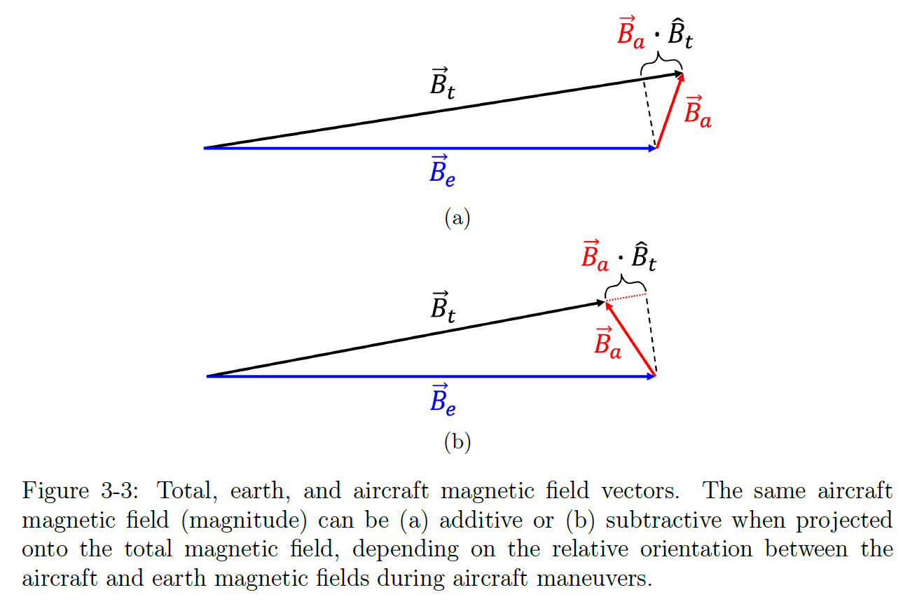
Organizing the above equation, we can obtain the vector form of the total constraint relationship relative to the model parameters.
\[|\vec{B}_t|-|\vec{B}_e|=\vec{\delta}^T\boldsymbol{\beta}\]where \(\vec{\delta}\) is calculated by
\[\vec{\delta}= \begin{bmatrix} \hat{B}_x \\ \hat{B}_y \\ \hat{B}_z \\ |\vec{B}_t|\hat{B}_x\hat{B}_x \\ |\vec{B}_t|\hat{B}_x\hat{B}_y \\ |\vec{B}_t|\hat{B}_x\hat{B}_z \\ |\vec{B}_t|\hat{B}_y\hat{B}_y \\ |\vec{B}_t|\hat{B}_y\hat{B}_z \\ |\vec{B}_t|\hat{B}_z\hat{B}_z \\ |\vec{B}_t|\hat{B}_x\dot{\hat{B}}_x \\ |\vec{B}_t|\hat{B}_x\dot{\hat{B}}_y \\ |\vec{B}_t|\hat{B}_x\dot{\hat{B}}_z \\ |\vec{B}_t|\hat{B}_y\dot{\hat{B}}_x \\ |\vec{B}_t|\hat{B}_y\dot{\hat{B}}_y \\ |\vec{B}_t|\hat{B}_y\dot{\hat{B}}_z \\ |\vec{B}_t|\hat{B}_z\dot{\hat{B}}_x \\ |\vec{B}_t|\hat{B}_z\dot{\hat{B}}_y \\ |\vec{B}_t|\hat{B}_z\dot{\hat{B}}_z \\ \end{bmatrix}\]Assuming a time series of length \(N\), where each instance of \(\vec{\delta}\) forms an \(N\times18\) matrix \(\boldsymbol{A}\).
\[\boldsymbol{A}= \begin{bmatrix} \vec{\delta}_1^T \\ \vdots\\ \vec{\delta}_N^T \\ \end{bmatrix}\]并且令
\[\boldsymbol{B}_t= \begin{bmatrix} |\vec{B}_t|_1 \\ \vdots\\ |\vec{B}_t|_N \\ \end{bmatrix}\] \[\boldsymbol{B}_e= \begin{bmatrix} |\vec{B}_e|_1 \\ \vdots\\ |\vec{B}_e|_N \\ \end{bmatrix}\]then,
\[\boldsymbol{B}_t-\boldsymbol{B}_e=\boldsymbol{A}\boldsymbol{\beta}\]The above equation can be solved by the least-square algorithm.
\[\boldsymbol{\beta}=(\boldsymbol{A}^T\boldsymbol{A})^{-1}\boldsymbol{A}^T(\boldsymbol{B}_t-\boldsymbol{B}_e)\]Model parameter estimation based on component constraint
Consider the equation based on the component constraint
\[\vec{B}_e=\vec{B}_t- \left( \begin{bmatrix} \beta_1 \\ \beta_2\\ \beta_3 \end{bmatrix}+ \begin{bmatrix} \beta_4 & \beta_5 & \beta_6 \\ \beta_5 & \beta_7 & \beta_8 \\ \beta_6 & \beta_8 & \beta_9 \end{bmatrix} |\vec{B}_t| \hat{B}_t+ \begin{bmatrix} \beta_{10} & \beta_{11} & \beta_{12} \\ \beta_{13} & \beta_{14} & \beta_{15} \\ \beta_{16} & \beta_{17} & \beta_{18} \end{bmatrix} |\vec{B}_t| \dot{\hat{B}}_t \right)\]Based on the model parameter form described earlier, organizing the above equation yields the vector form based on component relationships.
\[\vec{B}_t-\vec{B}_e=\Lambda\boldsymbol{\beta}\]The \(3\times18\) coefficient matrix is represented by
\[\Lambda= \begin{bmatrix} \lambda_1 & \lambda_2 & \lambda_3 \end{bmatrix}\]with
\[\lambda_1=\boldsymbol{I}_{3\times3}\] \[\lambda_2= \begin{bmatrix} |\vec{B}_t|\hat{B}_x & |\vec{B}_t|\hat{B}_y & |\vec{B}_t|\hat{B}_z & 0 & 0 & 0 \\ 0 & |\vec{B}_t|\hat{B}_x & 0 & |\vec{B}_t|\hat{B}_y & |\vec{B}_t|\hat{B}_z & 0 \\ 0 & 0 & |\vec{B}_t|\hat{B}_x & 0 & |\vec{B}_t|\hat{B}_y & |\vec{B}_t|\hat{B}_z \\ \end{bmatrix}\] \[\lambda_3= \begin{bmatrix} |\vec{B}_t|\dot{\hat{B}}_x & |\vec{B}_t|\dot{\hat{B}}_y & |\vec{B}_t|\dot{\hat{B}}_z & 0 & 0 & 0 & 0 & 0 & 0 \\ 0 & 0 & 0 & |\vec{B}_t|\dot{\hat{B}}_x & |\vec{B}_t|\dot{\hat{B}}_y & |\vec{B}_t|\dot{\hat{B}}_z & 0 & 0 & 0 \\ 0 & 0 & 0 & 0 & 0 & 0 & |\vec{B}_t|\dot{\hat{B}}_x & |\vec{B}_t|\dot{\hat{B}}_y & |\vec{B}_t|\dot{\hat{B}}_z \\ \end{bmatrix}\]Similarly, for a time series of length \(N\), a \(3N\times18\) coefficient matrix \(\boldsymbol{A}\) can be constructed.
\[\boldsymbol{A}= \begin{bmatrix} \Lambda_1 \\ \vdots\\ \Lambda_N \\ \end{bmatrix}\]let
\[\boldsymbol{B}_t= \begin{bmatrix} \vec{B}_{t1} \\ \vdots\\ \vec{B}_{tN} \\ \end{bmatrix}\] \[\boldsymbol{B}_e= \begin{bmatrix} \vec{B}_{e1} \\ \vdots\\ \vec{B}_{eN} \\ \end{bmatrix}\]then
\[\boldsymbol{B}_t-\boldsymbol{B}_e=\boldsymbol{A}\boldsymbol{\beta}\]The least-square algorithm is used for the estimation.
\[\boldsymbol{\beta}=(\boldsymbol{A}^T\boldsymbol{A})^{-1}\boldsymbol{A}^T(\boldsymbol{B}_t-\boldsymbol{B}_e)\]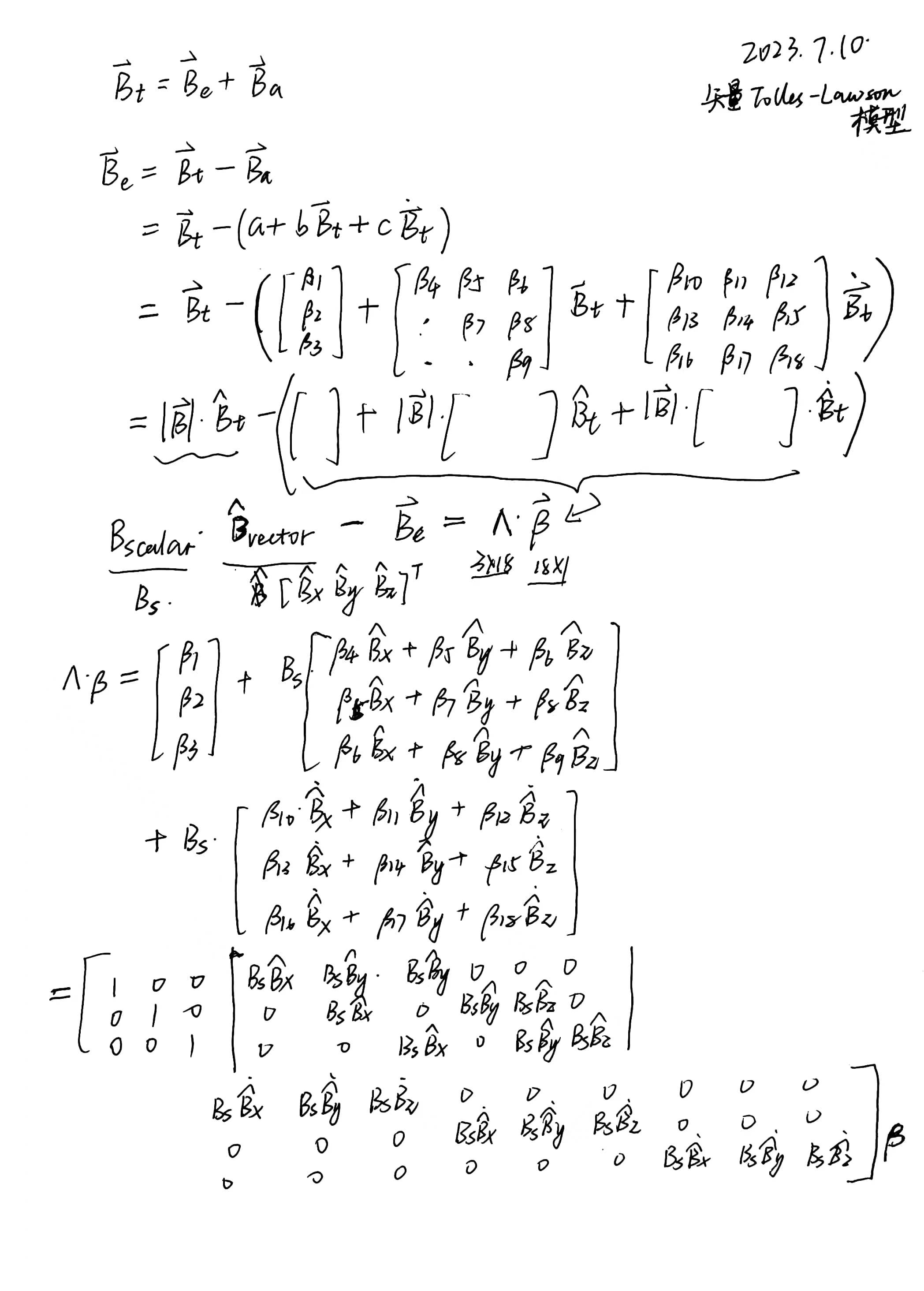
Component Compensation for Triaxial Magnetometer
After obtaining \(\boldsymbol{\beta}\) using the model parameter estimation method based on total constraint or component constraint, the vector magnetic compensation process can be carried out using the following equation.
\[\vec{B}_e=\vec{B}_t-\Lambda\boldsymbol{\beta}\]Acquisition of geomagnetic field calibration signals
In the process of model parameter estimation described earlier, both \(\vec{B}_t\) and \(\boldsymbol{\beta}\) come from measurements of scalar and vector magnetometers, while the source of the geomagnetic field \(\vec{B}_e\) requires further discussion.
Source 1: External Installation of Magnetometer (Ground Truth)
During calibration flights (magnetic compensation model fitting data collection), scalar and vector magnetic measurement systems are installed externally to synchronously capture ground truth geomagnetic field values at each moment. These values are used for model parameter estimation and compensation accuracy testing.
Comparing to the map values is not done in most of this work, since the tail stinger measurement is considered to be a better “truth” measurement as it was measured at the same time and avoids map errors.
ref. A. R. Gnadt, “Advanced Aeromagnetic Compensation Models for Airborne Magnetic Anomaly Navigation,” Massachusetts Institute of Technology, 2022.
Source 2: High-Precision Geomagnetic Reference Map
Currently not applicable and does not provide vector geomagnetic field information.
The map-based calibration, is less common in the literature, but more intuitive. This calibration method flies through a high-quality magnetic anomaly map (with GPS) and calibrates the system measurements such that they most closely match the magnetic anomaly map. This method requires highly accurate magnetic anomaly maps but can produce the best results given the navigation system is also using this map to navigate. This method cannot produce calibration errors smaller than the errors which exist in the magnetic map-products being used.
ref. A. J. Canciani, “Magnetic Navigation on an F-16 Aircraft Using Online Calibration,” in IEEE Transactions on Aerospace and Electronic Systems, vol. 58, no. 1, pp. 420-434.
Source 3: BPF “Trick”
During calibration flights, areas with minimal geomagnetic field variation are selected, and the drone performs various maneuvers. A band-pass filter is then used to filter out the geomagnetic field signal.
However, this approach is only suitable for the “model parameter estimation based on total constraint” method.
The “trick” is to use a bandpass finite impulse response filter (bpf).
The passband frequency range for the bandpass filter is carefully selected in order to remove nearly all of the earth field while keeping much of the aircraft field. In practice, a passband of 0.1-0.9 Hz has been found to perform well, since in this range the frequency content of the aircraft dominates the magnetic signal.
ref. A. R. Gnadt, “Advanced Aeromagnetic Compensation Models for Airborne Magnetic Anomaly Navigation,” Massachusetts Institute of Technology, 2022.
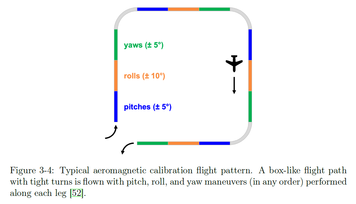
Calibration Flight
During the calibration flight, the aircraft performs a series of specific roll, pitch, and yaw maneuvers to collect measurements required for model parameter estimation.
According to the “Aviation Magnetometry Technology Standards”, the aircraft’s magnetic field compensation flight method uses a square flight pattern. On each leg, the aircraft performs pitch, roll, and yaw maneuvers within a certain angle range.
Calibration flights are typically conducted at high altitudes, where the geomagnetic gradient is relatively small. However, this requirement primarily applies to the geomagnetic field filtering method based on the BPF “trick” for filtering out the constant magnetic field. For the other two geomagnetic field sources, the requirement for geomagnetic gradient can be relatively relaxed.
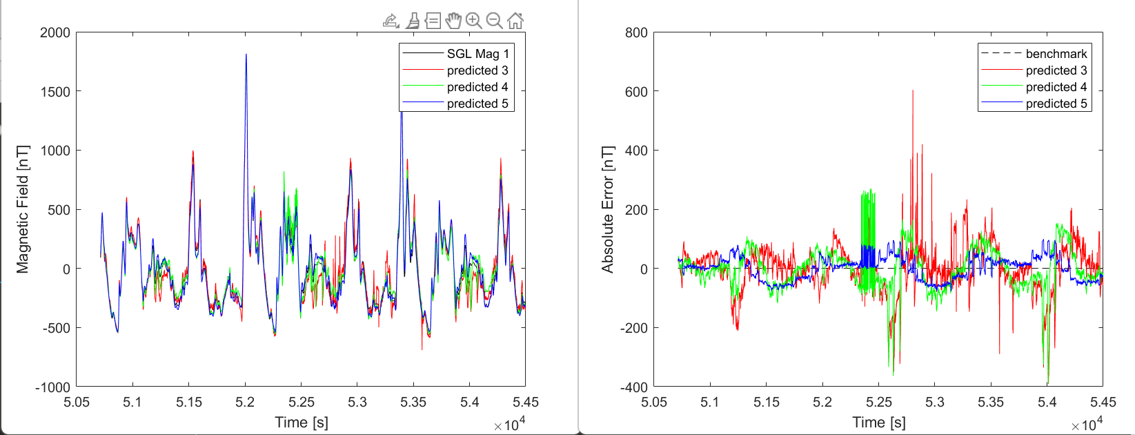
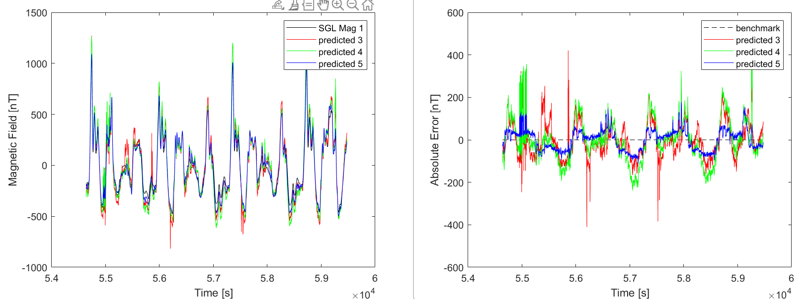
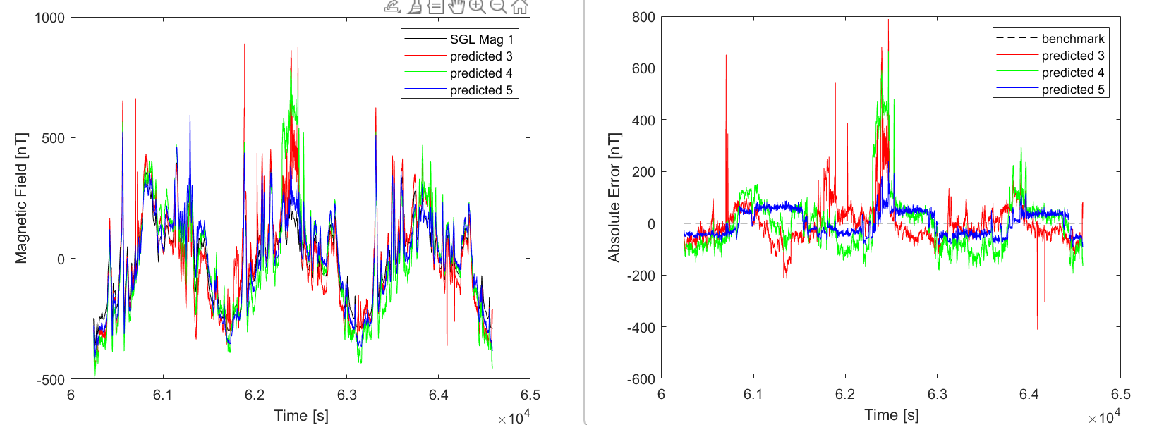
Experiments
mag 3 - ensemble rmse on 1003.020000 = 82.502527
mag 4 - ensemble rmse on 1003.020000 = 70.903014
mag 5 - ensemble rmse on 1003.020000 = 38.197016
mag 3 - ensemble rmse on 1003.040000 = 83.237522
mag 4 - ensemble rmse on 1003.040000 = 102.557146
mag 5 - ensemble rmse on 1003.040000 = 49.126008
mag 3 - ensemble rmse on 1003.080000 = 87.115366
mag 4 - ensemble rmse on 1003.080000 = 118.260125
mag 5 - ensemble rmse on 1003.080000 = 48.884029
Related Links
patent:
code: